Two-way ANOVA Introduction to Factorial Designs and their Analysis

Two-way ANOVA Introduction to Factorial Designs and their Analysis

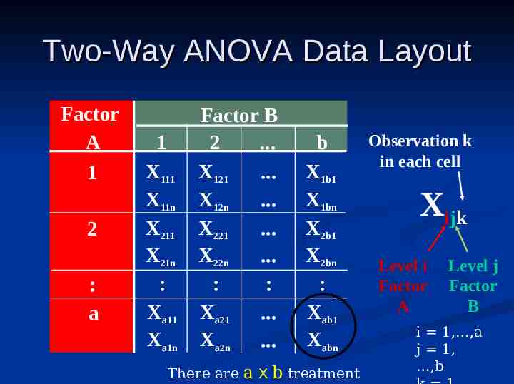
Two-Way ANOVA Data Layout Factor A 1 2 : a 1 X111 X11n X211 X21n : Xa11 Xa1n Factor B 2 . X121 . X12n . X221 . X22n . : : Xa21 . Xa2n . b X1b1 X1bn X2b1 X2bn : Xab1 Xabn There are a X b treatment Observation k in each cell Xijk Level i Factor A Level j Factor B i 1, ,a j 1, ,b

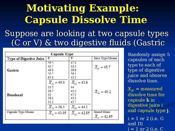
Motivating Example: Capsule Dissolve Time Suppose are looking at two capsule types (C or V) & two digestive fluids (Gastric or Duodenal) Randomly assign 5 capsules of each type to each of type of digestive juice and observe dissolve time. Xijk measured dissolve time for capsule k in digestive juice i and capsule type j. i 1 or 2 (i.e. G and D) j 1 or 2 (i.e. C

Questions of Interest What effect does capsule type have on the time to dissolve? What effect does fluid type have on the time to dissolve? Do both capsule types dissolve in the same manner in the two different fluid types?

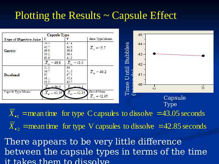
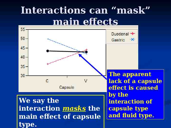
Time Until Bubbles (seconds) Plotting the Results Capsule Effect Capsule Type X 1 mean time for type C capsules to dissolve 43.05 seconds X 2 mean time for type V capsules to dissolve 42.85 seconds There appears to be very little difference between the capsule types in terms of the time

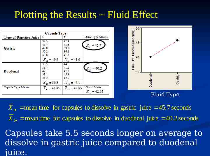
Plotting the Results Fluid Effect Fluid Type X 1 mean time for capsules to dissolve in gastric juice 45.7 seconds X 2 mean time for capsules to dissolve in duodenal juice 40.2 seconds Capsules take 5.5 seconds longer on average to dissolve in gastric juice compared to duodenal juice.

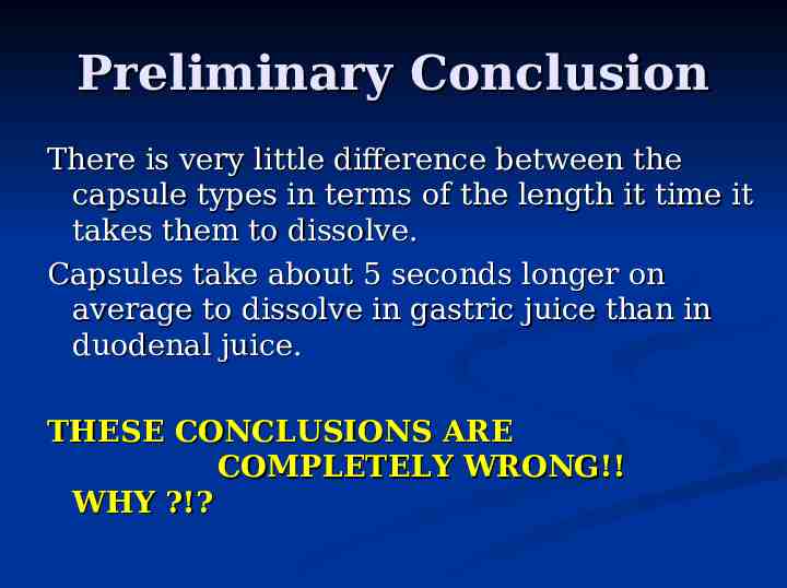
Preliminary Conclusion There is very little difference between the capsule types in terms of the length it time it takes them to dissolve. Capsules take about 5 seconds longer on average to dissolve in gastric juice than in duodenal juice. THESE CONCLUSIONS ARE COMPLETELY WRONG!! WHY ?!?

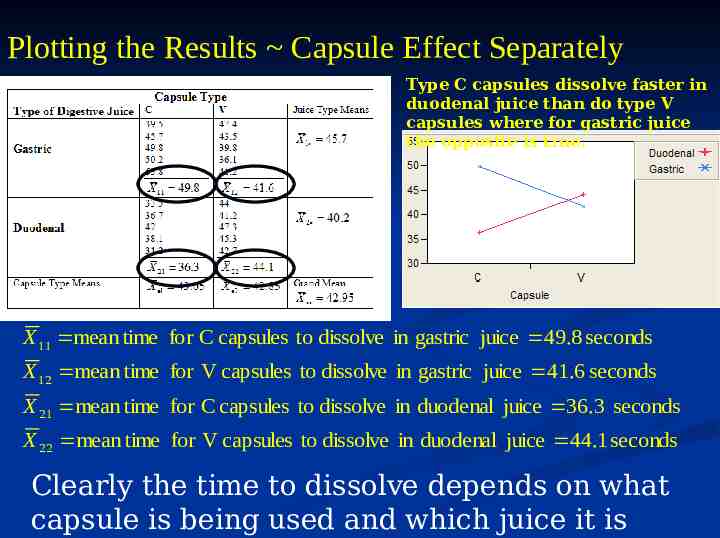
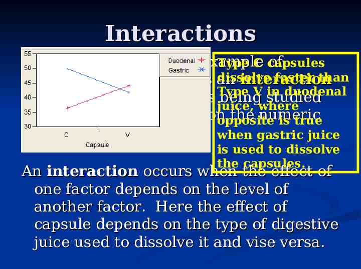
Plotting the Results Capsule Effect Separately Type C capsules dissolve faster in duodenal juice than do type V capsules where for gastric juice the opposite is true. X 11 mean time for C capsules to dissolve in gastric juice 49.8 seconds X 12 mean time for V capsules to dissolve in gastric juice 41.6 seconds X 21 mean time for C capsules to dissolve in duodenal juice 36.3 seconds X 22 mean time for V capsules to dissolve in duodenal juice 44.1 seconds Clearly the time to dissolve depends on what capsule is being used and which juice it is

Interactions The capsule study is an example of Type C capsules dissolve faster than situation where there is an interaction V in duodenal between the two factors Type being studied juice, where in terms of their effect on the numeric opposite is true response. when gastric juice is used to dissolve the capsules. An interaction occurs when the effect of one factor depends on the level of another factor. Here the effect of capsule depends on the type of digestive juice used to dissolve it and vise versa.

Interactions can “mask” main effects We say the interaction masks the main effect of capsule type. The apparent lack of a capsule effect is caused by the interaction of capsule type and fluid type.

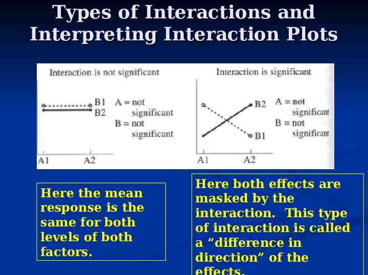
Types of Interactions and Interpreting Interaction Plots Here the mean response is the same for both levels of both factors. Here both effects are masked by the interaction. This type of interaction is called a “difference in direction” of the

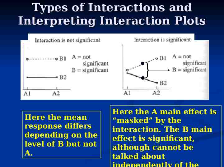
Types of Interactions and Interpreting Interaction Plots Here the mean response differs depending on the level of B but not A. Here the A main effect is “masked” by the interaction. The B main effect is significant, although cannot be talked about

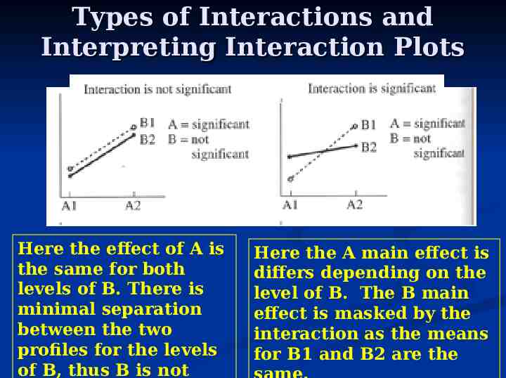
Types of Interactions and Interpreting Interaction Plots Here the effect of A is the same for both levels of B. There is minimal separation between the two profiles for the levels of B, thus B is not Here the A main effect is differs depending on the level of B. The B main effect is masked by the interaction as the means for B1 and B2 are the

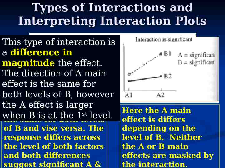
Types of Interactions and Interpreting Interaction Plots This type of interaction is a difference in magnitude the effect. The direction of A main effect is the same for both levels of B, however the A effect is larger Here the effect of A is Here the A main st when B isfor at both the 1levels level. effect is differs the same of B and vise versa. The response differs across the level of both factors and both differences suggest significant A & depending on the level of B. Neither the A or B main effects are masked by the interaction.

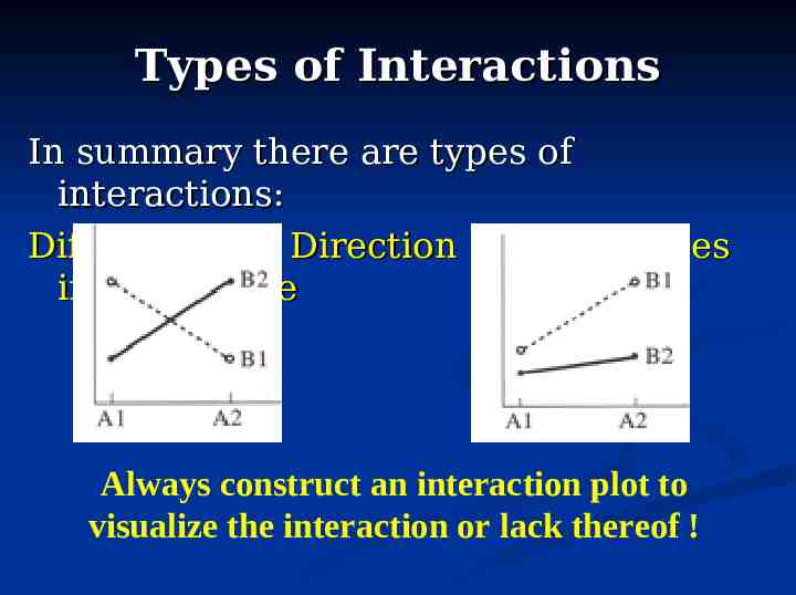
Types of Interactions In summary there are types of interactions: Differences in Direction Differences in Magnitude Always construct an interaction plot to visualize the interaction or lack thereof !

Questions of Interest Generally, the questions of interest here (i.e. hypotheses to be tested) concern three questions regarding the potential effects of the factors on the response variable. Question 1: Do the effects that factors A and B have on the response variable interact, i.e. is there a significant interaction between factors A and B ?

Questions of Interest If we conclude there is a significant interaction then we conclude the effects of both factors A and B are significant! When we have an interaction we cannot consider the effect of either factor independently of the other, therefore both factors matter.

Questions of Interest If there is not a significant interaction effect then we can consider the main effects separately, i.e. we ask the following: Question 2: Does factor A alone have a significant effect? Question 3: Does factor B alone have a significant effect?

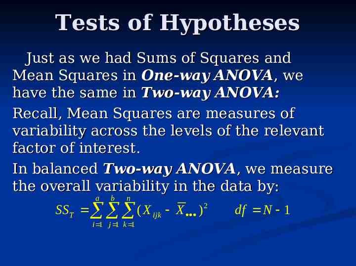
Tests of Hypotheses Just as we had Sums of Squares and Mean Squares in One-way ANOVA, we have the same in Two-way ANOVA: Recall, Mean Squares are measures of variability across the levels of the relevant factor of interest. In balanced Two-way ANOVA, we measure the overall variability in the data by: a b n SS T ( X ijk X ) 2 i 1 j 1 k 1 df N 1

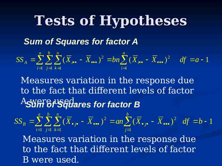
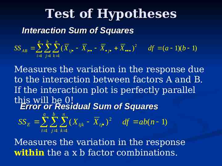
Tests of Hypotheses Sum of Squares for factor A a b n a SS A ( X i X ) 2 bn ( X i X ) 2 i 1 j 1 k 1 df a 1 i 1 Measures variation in the response due to the fact that different levels of factor ASum were ofused. Squares for factor B a b n b SS B ( X j X ) an ( X j X ) 2 df b 1 i 1 j 1 k 1 2 j 1 Measures variation in the response due to the fact that different levels of factor B were used.

Test of Hypotheses Interaction Sum of Squares a b n SS AB ( X ij X i X j X ) 2 df (a 1)(b 1) i 1 j 1 k 1 Measures the variation in the response due to the interaction between factors A and B. If the interaction plot is perfectly parallel this will be 0! Error or Residual Sum of Squares a b n SS E ( X ijk X ij ) 2 df ab(n 1) i 1 j 1 k 1 Measures the variation in the response within the a x b factor combinations.

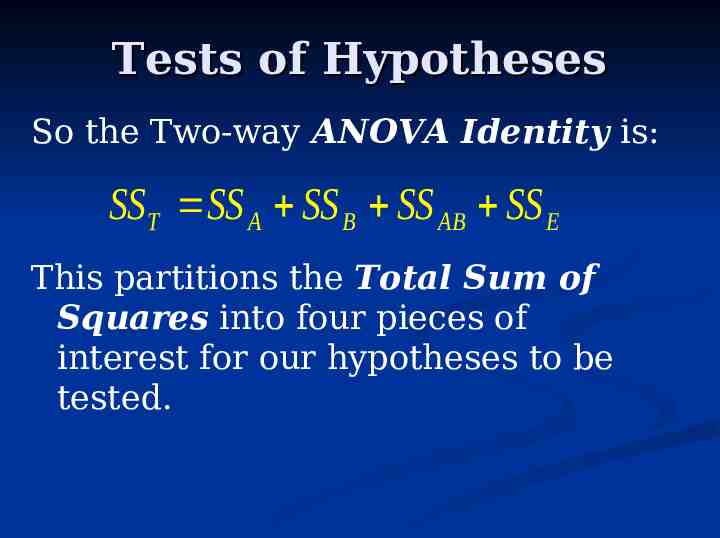
Tests of Hypotheses So the Two-way ANOVA Identity is: SST SS A SS B SS AB SS E This partitions the Total Sum of Squares into four pieces of interest for our hypotheses to be tested.

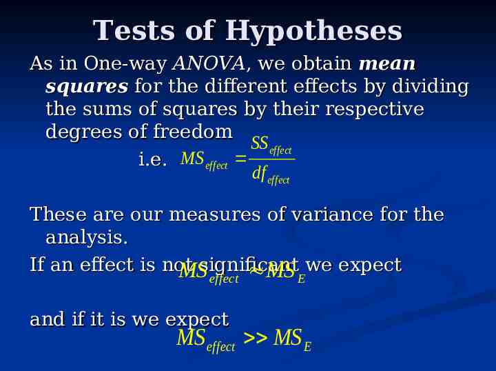
Tests of Hypotheses As in One-way ANOVA, we obtain mean squares for the different effects by dividing the sums of squares by their respective degrees of freedom SS effect i.e. MS effect df effect These are our measures of variance for the analysis. If an effect is not MSsignificant MS we expect effect and if it is we expect E MS effect MS E

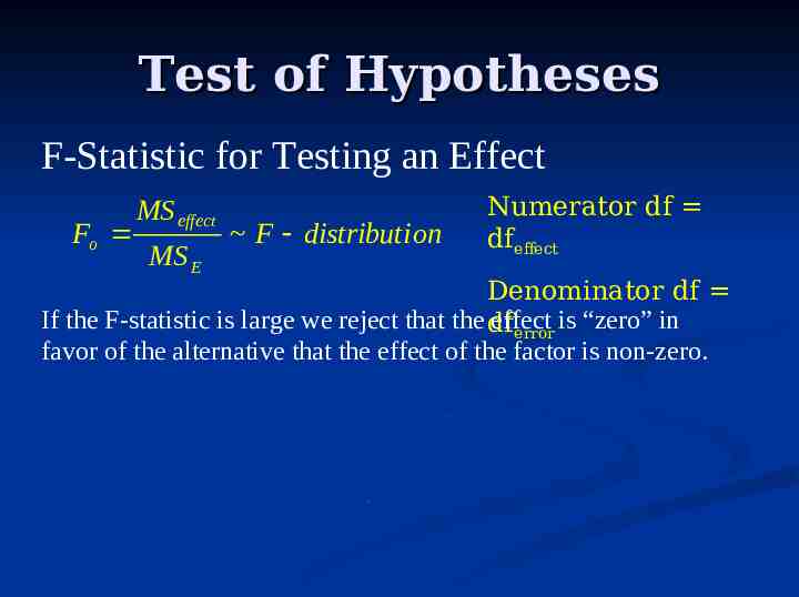
Test of Hypotheses F-Statistic for Testing an Effect Fo MS effect MS E F distributi on Numerator df dfeffect Denominator df If the F-statistic is large we reject that the df effect is “zero” in error favor of the alternative that the effect of the factor is non-zero.

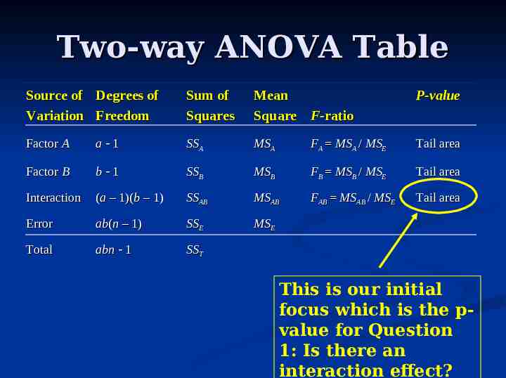
Two-way ANOVA Table Source of Degrees of Variation Freedom Sum of Squares Mean Square F-ratio P-value Factor A a 1 SSA MSA FA MSA / MSE Tail area Factor B b 1 SSB MSB FB MSB / MSE Tail area Interaction (a – 1)(b – 1) SSAB MSAB FAB MSAB / MSE Tail area Error ab(n – 1) SSE MSE Total abn 1 SST This is our initial focus which is the pvalue for Question 1: Is there an interaction effect?

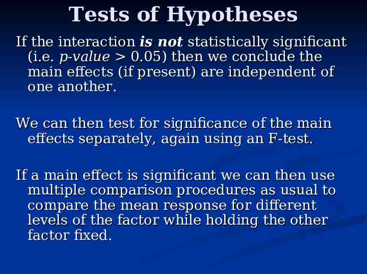
Tests of Hypotheses If the interaction is not statistically significant (i.e. p-value 0.05) then we conclude the main effects (if present) are independent of one another. We can then test for significance of the main effects separately, again using an F-test. If a main effect is significant we can then use multiple comparison procedures as usual to compare the mean response for different levels of the factor while holding the other factor fixed.

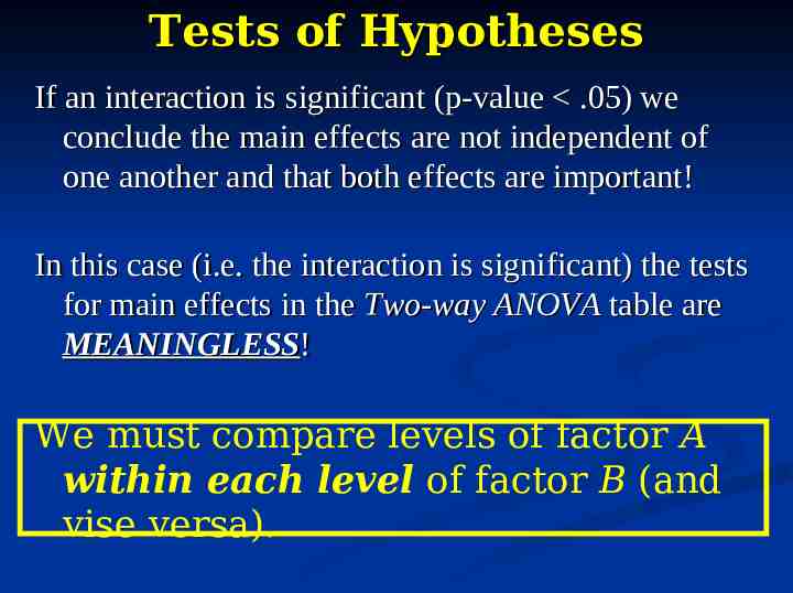
Tests of Hypotheses If an interaction is significant (p-value .05) we conclude the main effects are not independent of one another and that both effects are important! In this case (i.e. the interaction is significant) the tests for main effects in the Two-way ANOVA table are MEANINGLESS! We must compare levels of factor A within each level of factor B (and vise versa).

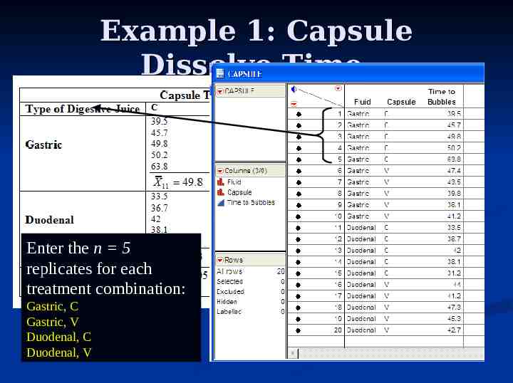
Example 1: Capsule Dissolve Time Enter the n 5 replicates for each treatment combination: Gastric, C Gastric, V Duodenal, C Duodenal, V

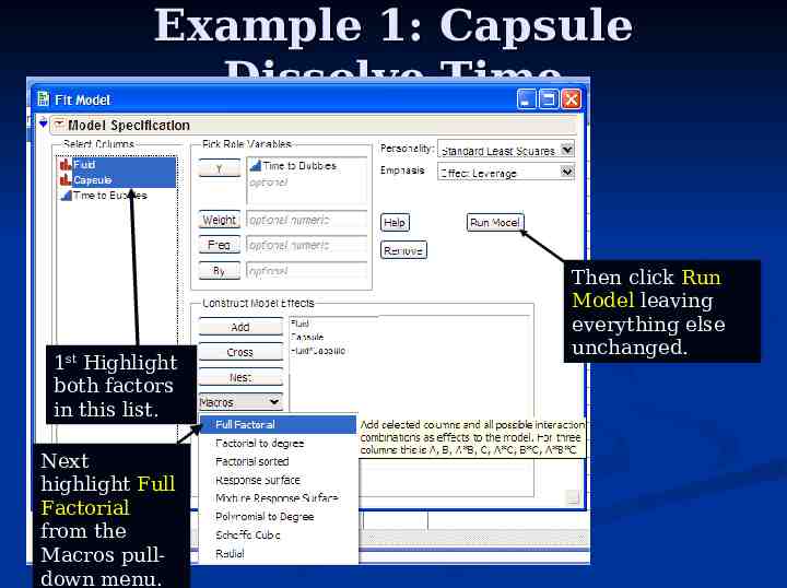
Example 1: Capsule Dissolve Time 1st Highlight both factors in this list. Next highlight Full Factorial from the Macros pulldown menu. Then click Run Model leaving everything else unchanged.

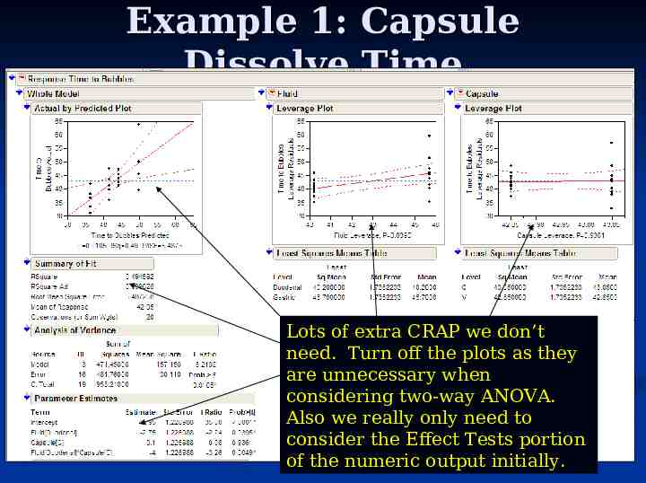
Example 1: Capsule Dissolve Time Lots of extra CRAP we don’t need. Turn off the plots as they are unnecessary when considering two-way ANOVA. Also we really only need to consider the Effect Tests portion of the numeric output initially.

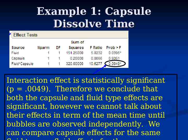
Example 1: Capsule Dissolve Time Interaction effect is statistically significant (p .0049). Therefore we conclude that both the capsule and fluid type effects are significant, however we cannot talk about their effects in term of the mean time until bubbles are observed independently. We can compare capsule effects for the same

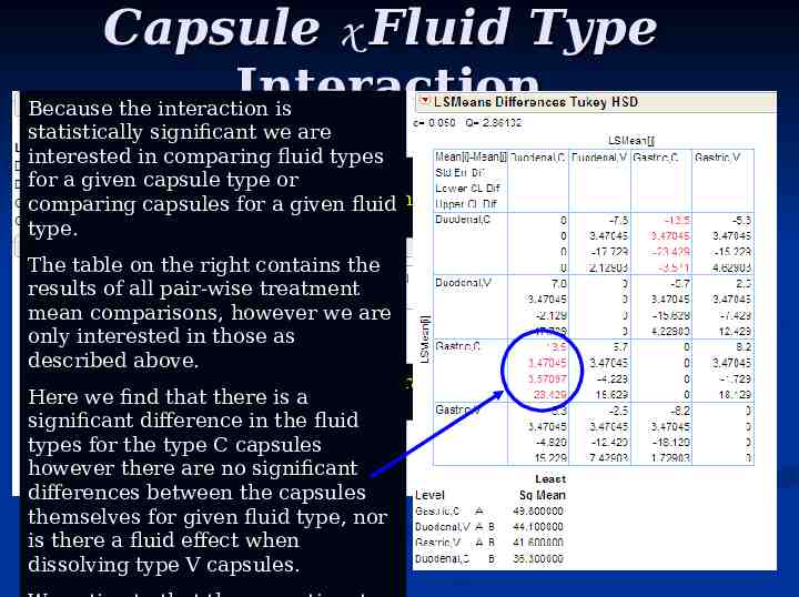
Capsule x Fluid Type Interaction Because the interaction is statistically significant we are interested in comparing fluid types Treatment for a given capsule type or comparing capsules for a combination given fluid means. type. The table on the right contains the results of all pair-wise treatment mean comparisons, however we are only interested in those as described above. Interaction Here we find that there is a Plot significant difference in the fluid types for the type C capsules however there are no significant differences between the capsules themselves for given fluid type, nor is there a fluid effect when dissolving type V capsules.

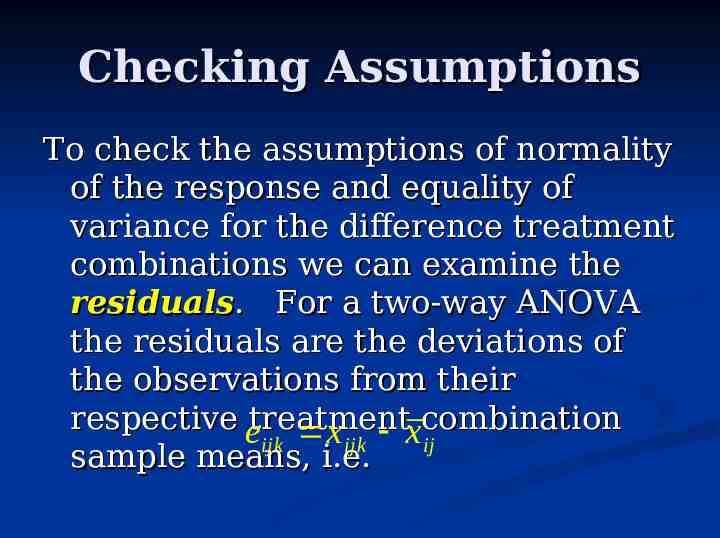
Checking Assumptions To check the assumptions of normality of the response and equality of variance for the difference treatment combinations we can examine the residuals. For a two-way ANOVA the residuals are the deviations of the observations from their respective etreatment combination ijk x ijk x ij sample means, i.e.

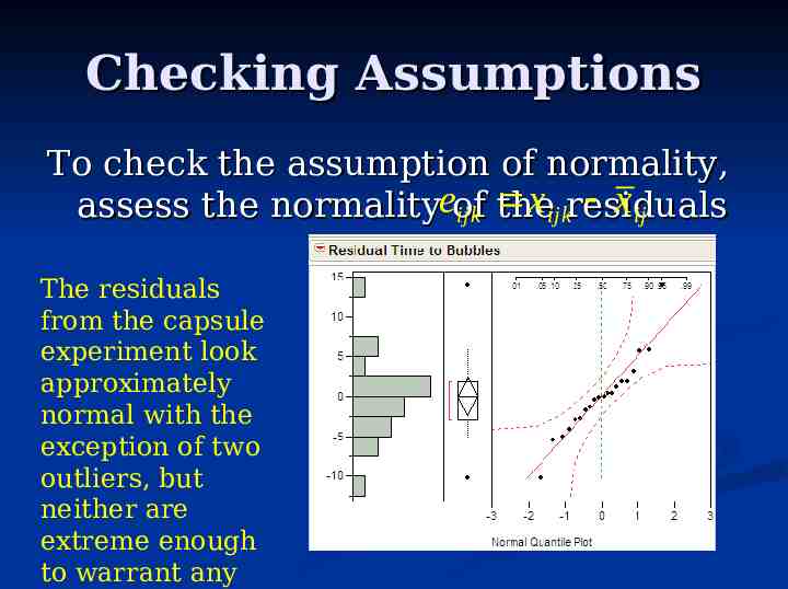
Checking Assumptions To check the assumption of normality, xijkresiduals xij assess the normalityeof the ijk The residuals from the capsule experiment look approximately normal with the exception of two outliers, but neither are extreme enough to warrant any

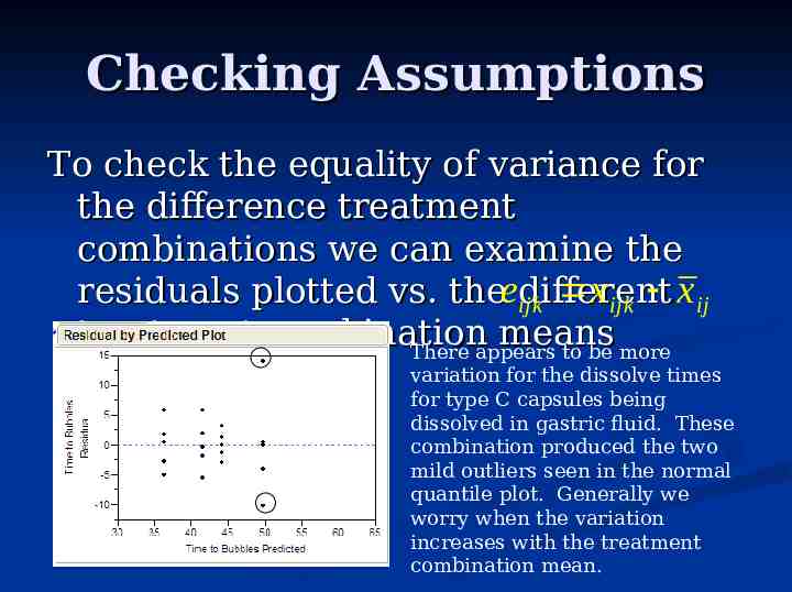
Checking Assumptions To check the equality of variance for the difference treatment combinations we can examine the xijk xij residuals plotted vs. theeijk different treatment combination means There appears to be more variation for the dissolve times for type C capsules being dissolved in gastric fluid. These combination produced the two mild outliers seen in the normal quantile plot. Generally we worry when the variation increases with the treatment combination mean.

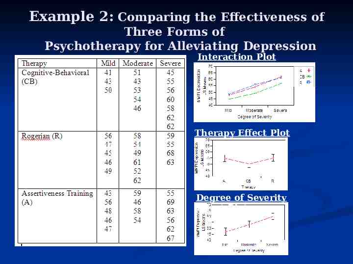
Example 2: Comparing the Effectiveness of Three Forms of Psychotherapy for Alleviating Depression Suppose that a clinical psychologist is interested in comparing the relative effectiveness of three forms of psychotherapy for alleviating depression. Fifteen individuals are randomly assigned to each of three treatment groups: cognitive-behavioral, Rogerian, and assertiveness training. The Depression Scale of MMPI serves as the response. The psychologist also wished to incorporate information about the patient’s severity of depression, so all subjects in the study were classified as having mild, moderate, or severe depression. Thus we have two factor of interest in this study: the treatment they received and the initial severity of their depression.

Example 2: Comparing the Effectiveness of Three Forms of Psychotherapy for Alleviating Depression Interaction Plot Therapy Effect Plot Degree of Severity Effect Plot

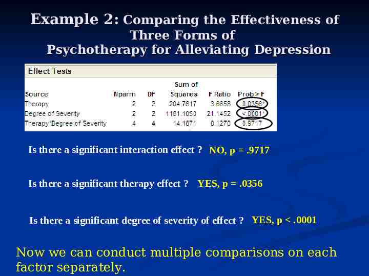
Example 2: Comparing the Effectiveness of Three Forms of Psychotherapy for Alleviating Depression Is there a significant interaction effect ? NO, p .9717 Is there a significant therapy effect ? YES, p .0356 Is there a significant degree of severity of effect ? YES, p .0001 Now we can conduct multiple comparisons on each factor separately.

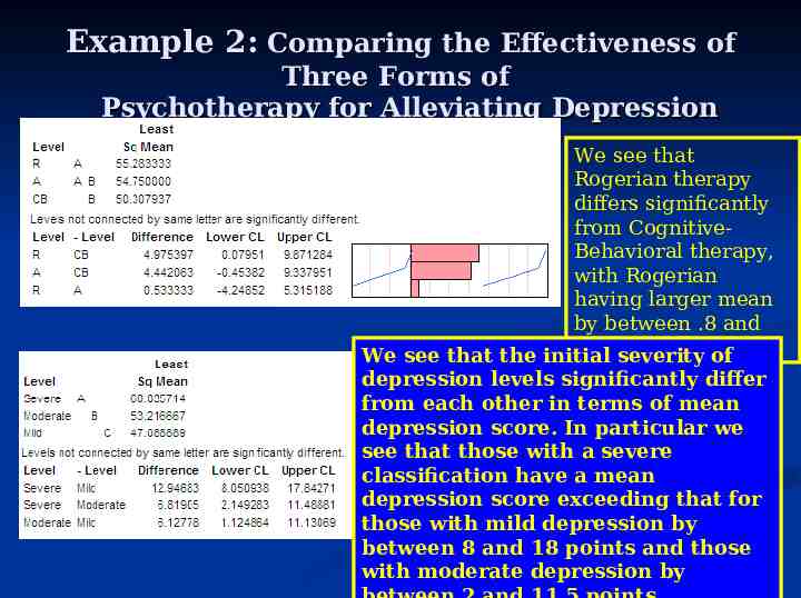
Example 2: Comparing the Effectiveness of Three Forms of Psychotherapy for Alleviating Depression We see that Rogerian therapy differs significantly from CognitiveBehavioral therapy, with Rogerian having larger mean by between .8 and 9.87severity units. of We see that the initial depression levels significantly differ from each other in terms of mean depression score. In particular we see that those with a severe classification have a mean depression score exceeding that for those with mild depression by between 8 and 18 points and those with moderate depression by

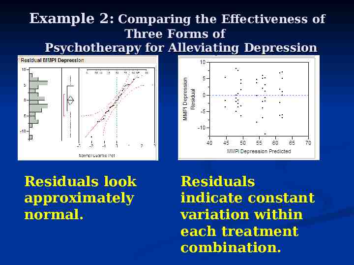
Example 2: Comparing the Effectiveness of Three Forms of Psychotherapy for Alleviating Depression Residuals look approximately normal. Residuals indicate constant variation within each treatment combination.

Summary These ideas can be extended to more than two factors. When interactions exist, the main effects are involved are important, but cannot discussed separately. Multiple comparisons can still be conducted