Topics in Computational Sustainability Optimization: Intro to

Topics in Computational Sustainability Optimization: Intro to Linear programming

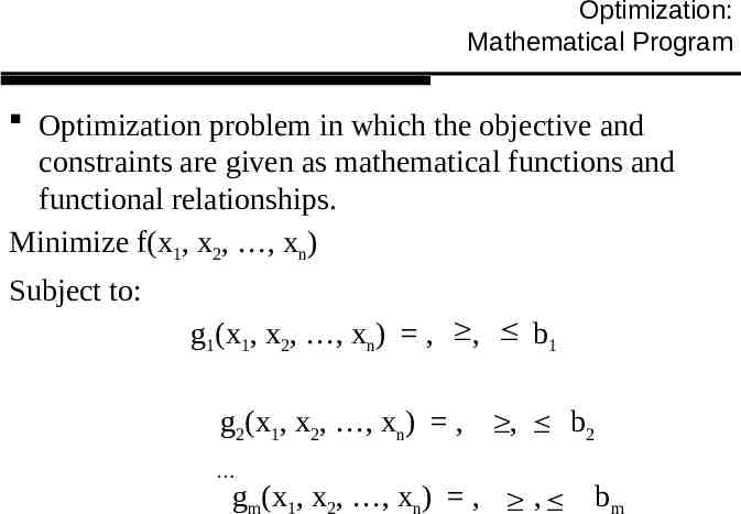
Optimization: Mathematical Program Optimization problem in which the objective and constraints are given as mathematical functions and functional relationships. Minimize f(x1, x2, , xn) Subject to: g1(x1, x2, , xn) , , b1 g2(x1, x2, , xn) , , b2 gm(x1, x2, , xn) , , bm

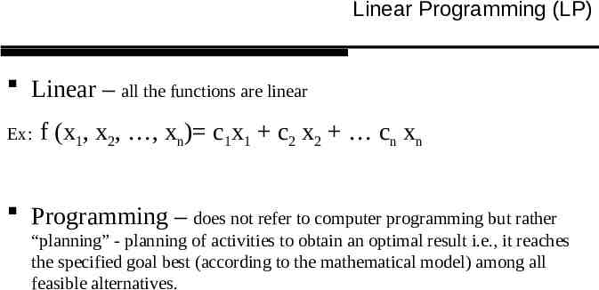
Linear Programming (LP) Linear – all the functions are linear Ex: f (x1, x2, , xn) c1x1 c2 x2 cn xn Programming – does not refer to computer programming but rather “planning” - planning of activities to obtain an optimal result i.e., it reaches the specified goal best (according to the mathematical model) among all feasible alternatives.

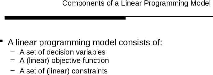
Components of a Linear Programming Model A linear programming model consists of: – A set of decision variables – A (linear) objective function – A set of (linear) constraints

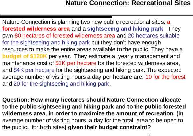
Nature Connection: Recreational Sites Nature Connection is planning two new public recreational sites: a forested wilderness area and a sightseeing and hiking park. They own 80 hectares of forested wilderness area and 20 hectares suitable for the sightseeing and hiking park but they don’t have enough resources to make the entire areas available to the public. They have a budget of 120K per year. They estimate a yearly management and maintenance cost of 1K per hectare for the forested wilderness area, and 4K per hectare for the sightseeing and hiking park. The expected average number of visiting hours a day per hectare are: 10 for the forest and 20 for the sightseeing and hiking park. Question: How many hectares should Nature Connection allocate to the public sightseeing and hiking park and to the public forested wilderness area, in order to maximize the amount of recreation, (in average number of visiting hours a day for the total area to be open to the public, for both sites) given their budget constraint? 5

Steps in setting up a LP 1. 2. 3. Determine and label the decision variables. Determine the objective and use the decision variables to write an expression for the objective function. Determine the constraints - feasible region. 1. 2. Determine the explicit constraints and write a functional expression for each of them. Determine the implicit constraints (e.g., nonnegativity constraints).

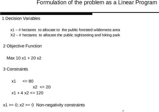
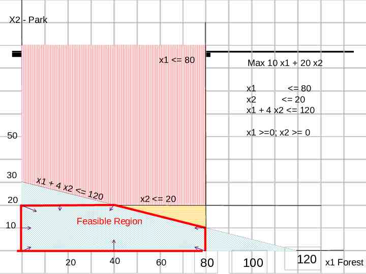
Formulation of the problem as a Linear Program 1 Decision Variables x1 – # hectares to allocate to the public forested wilderness area X2 – # hectares to allocate the public sightseeing and hiking park 2 Objective Function Max 10 x1 20 x2 3 Constraints x1 80 x2 20 x1 4 x2 120 x1 0; x2 0 Non-negativity constraints 7

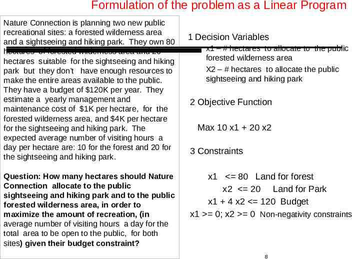
Formulation of the problem as a Linear Program Nature Connection is planning two new public recreational sites: a forested wilderness area and a sightseeing and hiking park. They own 80 hectares of forested wilderness area and 20 hectares suitable for the sightseeing and hiking park but they don’t have enough resources to make the entire areas available to the public. They have a budget of 120K per year. They estimate a yearly management and maintenance cost of 1K per hectare, for the forested wilderness area, and 4K per hectare for the sightseeing and hiking park. The expected average number of visiting hours a day per hectare are: 10 for the forest and 20 for the sightseeing and hiking park. Question: How many hectares should Nature Connection allocate to the public sightseeing and hiking park and to the public forested wilderness area, in order to maximize the amount of recreation, (in average number of visiting hours a day for the total area to be open to the public, for both sites) given their budget constraint? 1 Decision Variables x1 – # hectares to allocate to the public forested wilderness area X2 – # hectares to allocate the public sightseeing and hiking park 2 Objective Function Max 10 x1 20 x2 3 Constraints x1 80 Land for forest x2 20 Land for Park x1 4 x2 120 Budget x1 0; x2 0 Non-negativity constraints 8

X2 - Park x1 80 Max 10 x1 20 x2 x1 80 x2 20 x1 4 x2 120 x1 0; x2 0 50 30 x1 4 x2 20 1 20 10 Feasible Region 20 x2 20 40 60 80 100 120 x1 Forest

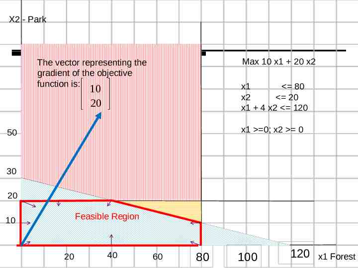
X2 - Park Max 10 x1 20 x2 The vector representing the gradient of the objective function is:é ù x1 80 x2 20 x1 4 x2 120 10 ê ú ë 20 û x1 0; x2 0 50 30 20 Feasible Region 10 20 40 60 80 100 120 x1 Forest

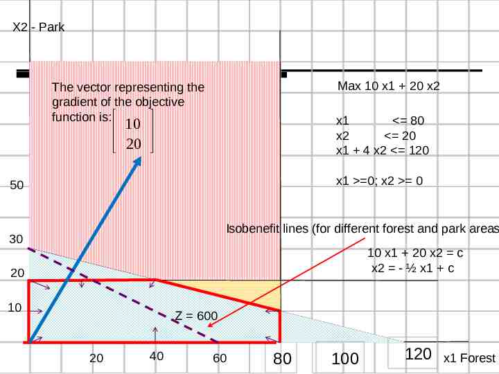
X2 - Park Max 10 x1 20 x2 The vector representing the gradient of the objective function is:é ù x1 80 x2 20 x1 4 x2 120 10 ê ú ë 20 û x1 0; x2 0 50 Isobenefit lines (for different forest and park areas 30 10 x1 20 x2 c x2 - ½ x1 c 20 10 Z 600 20 40 60 80 100 120 x1 Forest

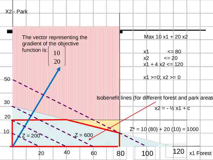
X2 - Park Max 10 x1 20 x2 The vector representing the gradient of the objective function is:é ù x1 80 x2 20 x1 4 x2 120 10 ê ú ë 20 û x1 0; x2 0 50 Isobenefit lines (for different forest and park areas 30 x2 - ½ x1 c 20 10 Z* 10 (80) 20 (10) 1000 Z 600 Z 200 20 40 60 80 100 120 x1 Forest

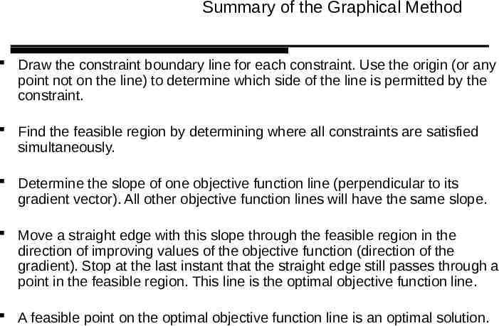
Summary of the Graphical Method Draw the constraint boundary line for each constraint. Use the origin (or any point not on the line) to determine which side of the line is permitted by the constraint. Find the feasible region by determining where all constraints are satisfied simultaneously. Determine the slope of one objective function line (perpendicular to its gradient vector). All other objective function lines will have the same slope. Move a straight edge with this slope through the feasible region in the direction of improving values of the objective function (direction of the gradient). Stop at the last instant that the straight edge still passes through a point in the feasible region. This line is the optimal objective function line. A feasible point on the optimal objective function line is an optimal solution.

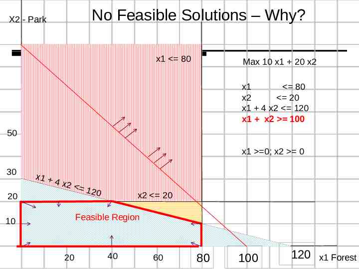
No Feasible Solutions – Why? X2 - Park x1 80 Max 10 x1 20 x2 x1 80 x2 20 x1 4 x2 120 x1 x2 100 50 x1 0; x2 0 30 x1 4 x2 20 1 20 10 Feasible Region 20 x2 20 40 60 80 100 120 x1 Forest

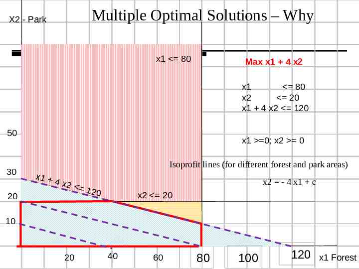
Multiple Optimal Solutions – Why X2 - Park x1 80 Max x1 4 x2 x1 80 x2 20 x1 4 x2 120 50 30 20 x1 0; x2 0 Isoprofit lines (for different forest and park areas) x1 4 x2 x2 - 4 x1 c 1 20 x2 20 10 20 40 60 80 100 120 x1 Forest

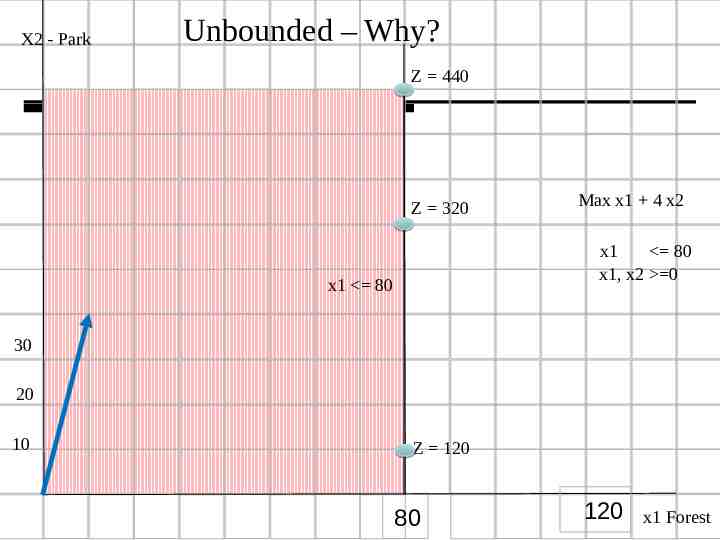
X2 - Park Unbounded – Why? Z 440 Z 320 Max x1 4 x2 x1 80 x1, x2 0 x1 80 30 20 10 Z 120 80 120 x1 Forest

Key Categories of LP problems: Resource-Allocation Problems Cost-benefit-trade-off problems Distribution-Network Problems Mixed problems

Second Example: Keeping the river clean Cost-benefit-trade-off problems Choose the mix of levels of various activities to achieve minimum acceptable levels for various benefits at a minimum cost.

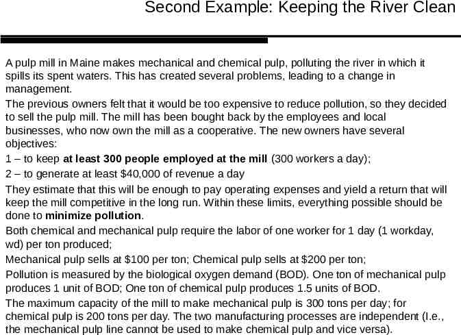
Second Example: Keeping the River Clean A pulp mill in Maine makes mechanical and chemical pulp, polluting the river in which it spills its spent waters. This has created several problems, leading to a change in management. The previous owners felt that it would be too expensive to reduce pollution, so they decided to sell the pulp mill. The mill has been bought back by the employees and local businesses, who now own the mill as a cooperative. The new owners have several objectives: 1 – to keep at least 300 people employed at the mill (300 workers a day); 2 – to generate at least 40,000 of revenue a day They estimate that this will be enough to pay operating expenses and yield a return that will keep the mill competitive in the long run. Within these limits, everything possible should be done to minimize pollution. Both chemical and mechanical pulp require the labor of one worker for 1 day (1 workday, wd) per ton produced; Mechanical pulp sells at 100 per ton; Chemical pulp sells at 200 per ton; Pollution is measured by the biological oxygen demand (BOD). One ton of mechanical pulp produces 1 unit of BOD; One ton of chemical pulp produces 1.5 units of BOD. The maximum capacity of the mill to make mechanical pulp is 300 tons per day; for chemical pulp is 200 tons per day. The two manufacturing processes are independent (I.e., the mechanical pulp line cannot be used to make chemical pulp and vice versa).

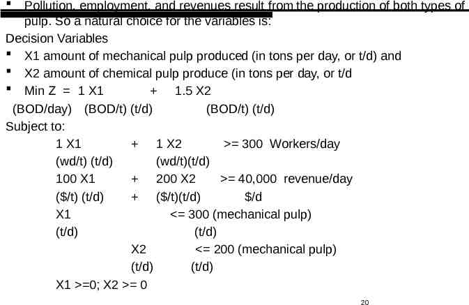
Pollution, employment, and revenues result from the production of both types of pulp. So a natural choice for the variables is: Decision Variables X1 amount of mechanical pulp produced (in tons per day, or t/d) and X2 amount of chemical pulp produce (in tons per day, or t/d Min Z 1 X1 1.5 X2 (BOD/day) (BOD/t) (t/d) (BOD/t) (t/d) Subject to: 1 X1 1 X2 300 Workers/day (wd/t) (t/d) (wd/t)(t/d) 100 X1 200 X2 40,000 revenue/day ( /t) (t/d) ( /t)(t/d) /d X1 300 (mechanical pulp) (t/d) (t/d) X2 200 (mechanical pulp) (t/d) (t/d) X1 0; X2 0 20

Distribution Network Problems

Distribution-Network Problem The International Hospital Share Organization is a non-profit organization that refurbishes a variety of used equipment for hospitals of developing countries at two international factories (F1 and F2). One of its products is a large X-Ray machine. Orders have been received from three large communities for the X-Ray machines.

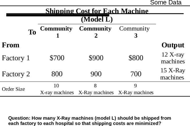
Some Data Shipping Cost for Each Machine (Model L) Community To 1 Community 2 Community 3 From Output Factory 1 700 900 800 Factory 2 800 900 700 Order Size 12 X-ray machines 15 X-Ray machines 10 8 9 X-ray machines X-Ray machines X-Ray machines Question: How many X-Ray machines (model L) should be shipped from each factory to each hospital so that shipping costs are minimized?

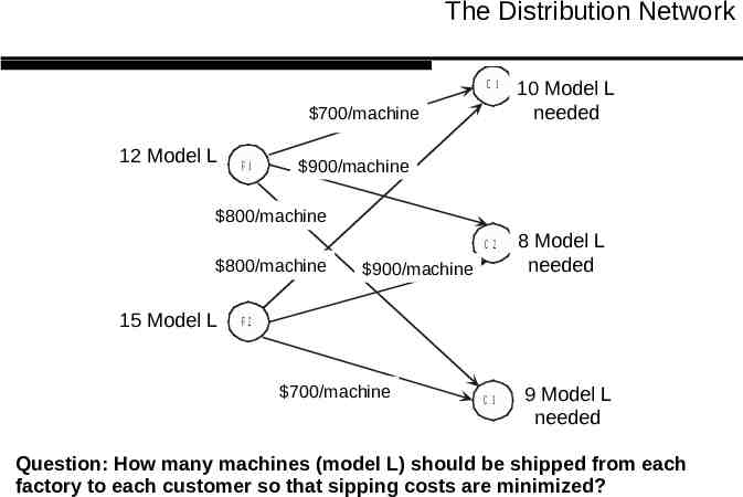
The Distribution Network C 1 700/machine 700/lathe 700/machine 12 Model 1 2 l a t hLe p ro d u c e d F1 900/machine 900/lathe 800/machine 800/lathe C 2 800/lathe 800/machine 1 5 l a t hLe s 15 Model p ro d u c ed 1 0 la th e s 10 L n e e d eModel d needed 900/lathe 900/machine th e s 88 l aModel L needed needed F2 700/lathe 700/machine C 3 9 9l a tModel hes needed L needed Question: How many machines (model L) should be shipped from each factory to each customer so that sipping costs are minimized?

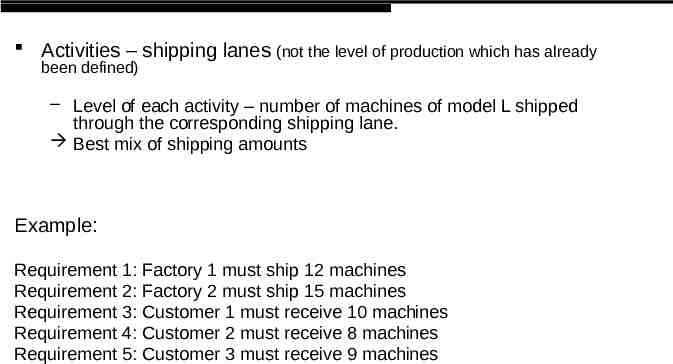
Activities – shipping lanes (not the level of production which has already been defined) – Level of each activity – number of machines of model L shipped through the corresponding shipping lane. Best mix of shipping amounts Example: Requirement 1: Factory 1 must ship 12 machines Requirement 2: Factory 2 must ship 15 machines Requirement 3: Customer 1 must receive 10 machines Requirement 4: Customer 2 must receive 8 machines Requirement 5: Customer 3 must receive 9 machines

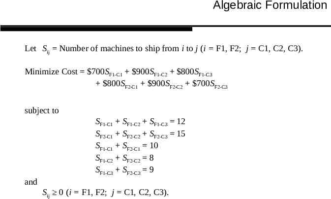
Algebraic Formulation Let Sij Number of machines to ship from i to j (i F1, F2; j C1, C2, C3). Minimize Cost 700SF1-C1 900SF1-C2 800SF1-C3 800SF2-C1 900SF2-C2 700SF2-C3 subject to SF1-C1 SF1-C2 SF1-C3 12 SF2-C1 SF2-C2 SF2-C3 15 SF1-C1 SF2-C1 10 SF1-C2 SF2-C2 8 SF1-C3 SF2-C3 9 and Sij 0 (i F1, F2; j C1, C2, C3).

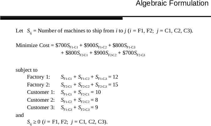
Algebraic Formulation Let Sij Number of machines to ship from i to j (i F1, F2; j C1, C2, C3). Minimize Cost 700SF1-C1 900SF1-C2 800SF1-C3 800SF2-C1 900SF2-C2 700SF2-C3 subject to Factory 1: SF1-C1 SF1-C2 SF1-C3 12 Factory 2: SF2-C1 SF2-C2 SF2-C3 15 Customer 1: SF1-C1 SF2-C1 10 Customer 2: SF1-C2 SF2-C2 8 Customer 3: SF1-C3 SF2-C3 9 and Sij 0 (i F1, F2; j C1, C2, C3).

Terminology and Notation 28

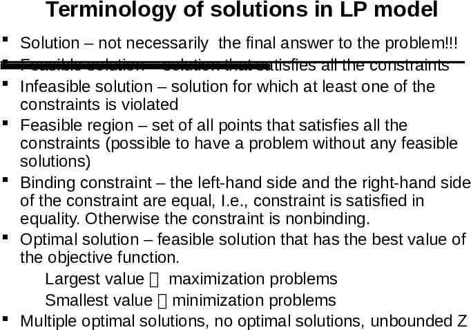
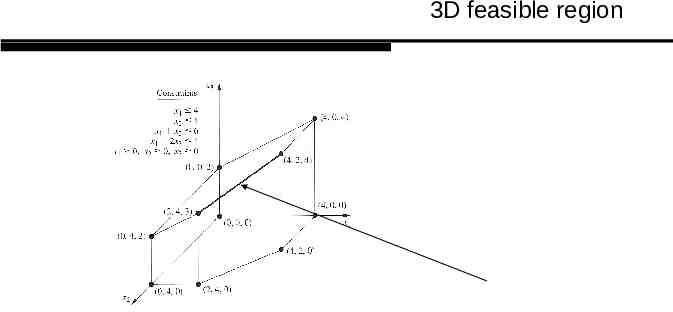
Terminology of solutions in LP model Solution – not necessarily the final answer to the problem!!! Feasible solution – solution that satisfies all the constraints Infeasible solution – solution for which at least one of the constraints is violated Feasible region – set of all points that satisfies all the constraints (possible to have a problem without any feasible solutions) Binding constraint – the left-hand side and the right-hand side of the constraint are equal, I.e., constraint is satisfied in equality. Otherwise the constraint is nonbinding. Optimal solution – feasible solution that has the best value of the objective function. Largest value maximization problems Smallest value minimization problems Multiple optimal solutions, no optimal solutions, unbounded Z

3D feasible region

Solving linear programs 31

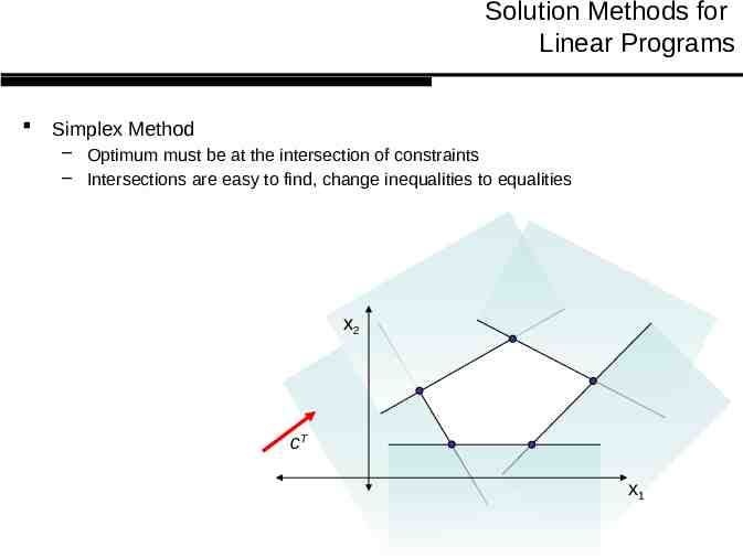
Solution Methods for Linear Programs Simplex Method – Optimum must be at the intersection of constraints – Intersections are easy to find, change inequalities to equalities x2 cT x1

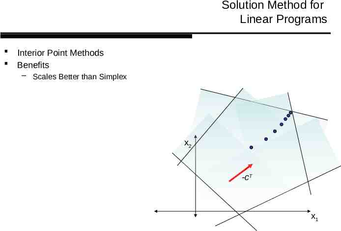
Solution Method for Linear Programs Interior Point Methods Benefits – Scales Better than Simplex x2 -cT x1

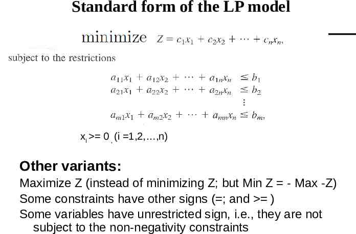
Standard form of the LP model xi 0 , (i 1,2, ,n) Other variants: Maximize Z (instead of minimizing Z; but Min Z - Max -Z) Some constraints have other signs ( ; and ) Some variables have unrestricted sign, i.e., they are not subject to the non-negativity constraints

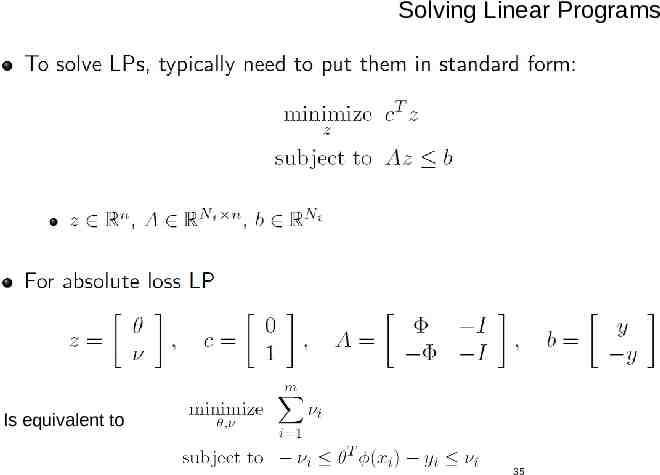
Solving Linear Programs Is equivalent to 35

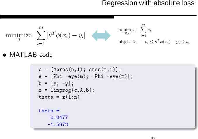
Regression with absolute loss 36