The Effects of Wal-Mart on Local Labor Markets David Neumark, Junfu

The Effects of Wal-Mart on Local Labor Markets David Neumark, Junfu Zhang, and Stephen Ciccarella

Why study Wal-Mart? Largest corporation in the world, with total revenues of 285 billion in 2005. Employs over 1.2 million workers in the United States, at about 3,600 stores. Just under 1% of total employment in the United States, and just under 10% of retail employment. Exceeds the number of high school teachers or middle school teachers, and is just under the size of the elementary school teacher workforce. Nation’s largest grocer, with a 19 percent market share, and its third-largest pharmacy, with a 16 percent market share.

Wal-Mart stores have generated opposition, based on many issues including: Wal-Mart eliminates more jobs than it creates Wal-Mart pulls down wages Wal-Mart increases burden on social programs Report by the Democratic Staff of the Committee on Education and the Workforce of the U.S. Congress claims that because of Wal-Mart’s low wages, an average Wal-Mart employee costs federal taxpayers an extra 2,103 in the form of tax credits or deductions, or public assistance such as healthcare, housing, and energy assistance. Obviously such effects depend on strong assumptions about what Wal-Mart workers would be doing if they weren’t working at Wal-Mart.

Wal-Mart disputes many of these claims: Vice President Bob McAdam has argued that there are many locations where Wal-Mart creates jobs in other businesses in addition to what Wal-Mart itself offers (PBS, 2004) The Wal-Mart web-site Walmartfacts.com trumpets the positive effects of Wal-Mart stores on retail jobs in the communities where stores open Advertisement run in the USA Today, The Wall Street Journal, and The New York Times on January 14, 2005, displayed an open letter from Lee Scott, Wal-Mart President and CEO, stating “This year, we plan to create more than 100,000 new jobs in the United States.”

What might we expect? Employment declines in retail are plausible, stemming from efficiency gains, lower staffing, etc. Broader employment declines seem unlikely, as labor moves to other uses, although frictions such as minimum wages could hamper adjustment for some workers. Source of wage declines less clear, given that Wal-Mart has to hire in a competitive labor market. Wal-Mart policies could lower wages in retail sector where stores open if there is redistribution of rents from workers, lowered union threat or competition with union sector, greater use of illegal workers, etc. Equilibrium wages could fall if lower prices affect real wages. Wages could also fall at suppliers, although we wouldn’t expect these effects in markets where stores locate.

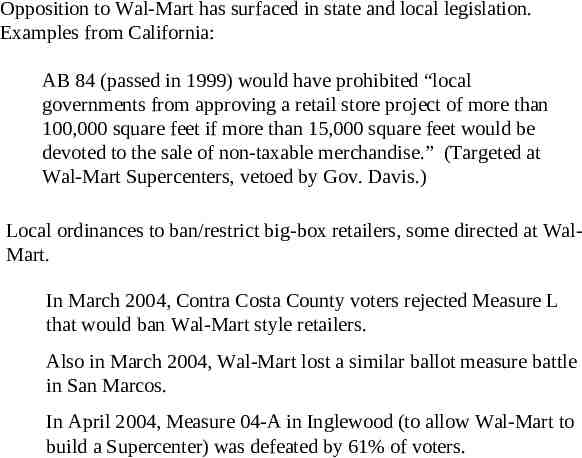
Opposition to Wal-Mart has surfaced in state and local legislation. Examples from California: AB 84 (passed in 1999) would have prohibited “local governments from approving a retail store project of more than 100,000 square feet if more than 15,000 square feet would be devoted to the sale of non-taxable merchandise.” (Targeted at Wal-Mart Supercenters, vetoed by Gov. Davis.) Local ordinances to ban/restrict big-box retailers, some directed at WalMart. In March 2004, Contra Costa County voters rejected Measure L that would ban Wal-Mart style retailers. Also in March 2004, Wal-Mart lost a similar ballot measure battle in San Marcos. In April 2004, Measure 04-A in Inglewood (to allow Wal-Mart to build a Supercenter) was defeated by 61% of voters.

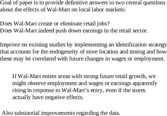
Goal of paper is to provide definitive answers to two central questions about the effects of Wal-Mart on local labor markets: Does Wal-Mart create or eliminate retail jobs? Does Wal-Mart indeed push down earnings in the retail sector. Improve on existing studies by implementing an identification strategy that accounts for the endogeneity of store location and timing and how these may be correlated with future changes in wages or employment. If Wal-Mart enters areas with strong future retail growth, we might observe employment and wages or earnings apparently rising in response to Wal-Mart’s entry, even if the stores actually have negative effects. Also substantial improvements regarding the data.

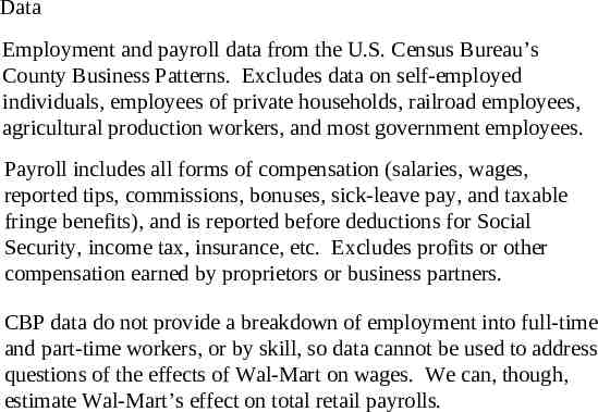
Data Employment and payroll data from the U.S. Census Bureau’s County Business Patterns. Excludes data on self-employed individuals, employees of private households, railroad employees, agricultural production workers, and most government employees. Payroll includes all forms of compensation (salaries, wages, reported tips, commissions, bonuses, sick-leave pay, and taxable fringe benefits), and is reported before deductions for Social Security, income tax, insurance, etc. Excludes profits or other compensation earned by proprietors or business partners. CBP data do not provide a breakdown of employment into full-time and part-time workers, or by skill, so data cannot be used to address questions of the effects of Wal-Mart on wages. We can, though, estimate Wal-Mart’s effect on total retail payrolls.

A sample: all observations (counties and years) with complete (nonsuppressed) employment and payroll data for aggregate retail, and in total. B sample: all observations in the A sample that also have complete data for the General Merchandising retail subsector (SIC 53 or NAICS 452) to which Wal-Mart belongs.

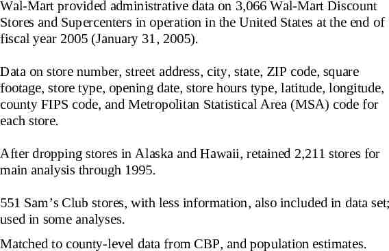
Wal-Mart provided administrative data on 3,066 Wal-Mart Discount Stores and Supercenters in operation in the United States at the end of fiscal year 2005 (January 31, 2005). Data on store number, street address, city, state, ZIP code, square footage, store type, opening date, store hours type, latitude, longitude, county FIPS code, and Metropolitan Statistical Area (MSA) code for each store. After dropping stores in Alaska and Hawaii, retained 2,211 stores for main analysis through 1995. 551 Sam’s Club stores, with less information, also included in data set; used in some analyses. Matched to county-level data from CBP, and population estimates.

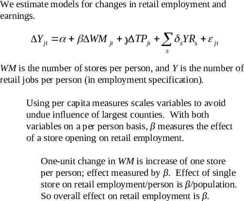
We estimate models for changes in retail employment and earnings. Y jt WM jt TPjt sYRs jt s WM is the number of stores per person, and Y is the number of retail jobs per person (in employment specification). Using per capita measures scales variables to avoid undue influence of largest counties. With both variables on a per person basis, β measures the effect of a store opening on retail employment. One-unit change in WM is increase of one store per person; effect measured by β. Effect of single store on retail employment/person is β/population. So overall effect on retail employment is β.

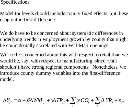
Specifications Model for levels should include county fixed effects, but these drop out in first-difference. We do have to be concerned about systematic differences in underlying trends in employment growth by county that might be coincidentally correlated with Wal-Mart openings We are less concerned about this with respect to retail than we would be, say, with respect to manufacturing, since retail shouldn’t have strong regional components. Nonetheless, we introduce county dummy variables into the first-difference model. Y jt WM jt TPjt i COi sYRs jt i s

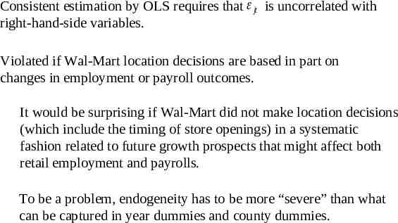
Consistent estimation by OLS requires that jt is uncorrelated with right-hand-side variables. Violated if Wal-Mart location decisions are based in part on changes in employment or payroll outcomes. It would be surprising if Wal-Mart did not make location decisions (which include the timing of store openings) in a systematic fashion related to future growth prospects that might affect both retail employment and payrolls. To be a problem, endogeneity has to be more “severe” than what can be captured in year dummies and county dummies.

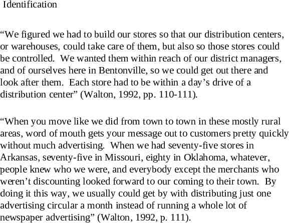
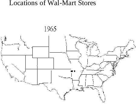
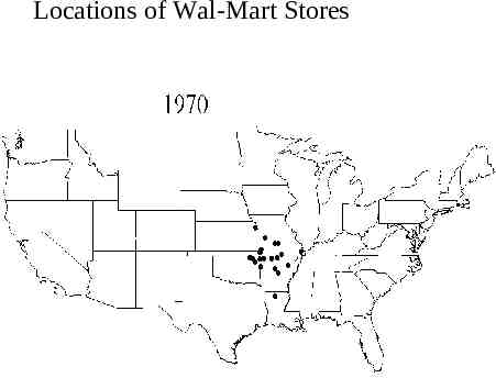
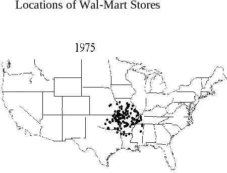
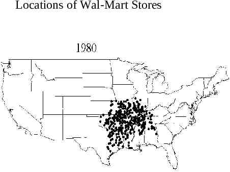
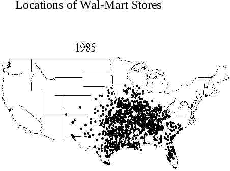
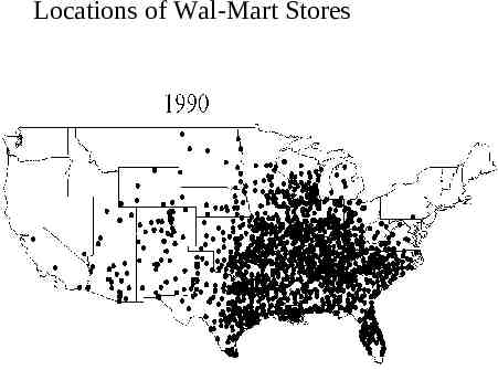
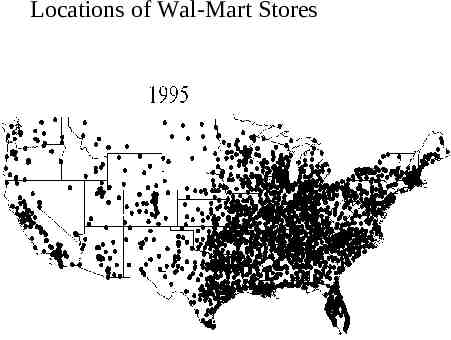
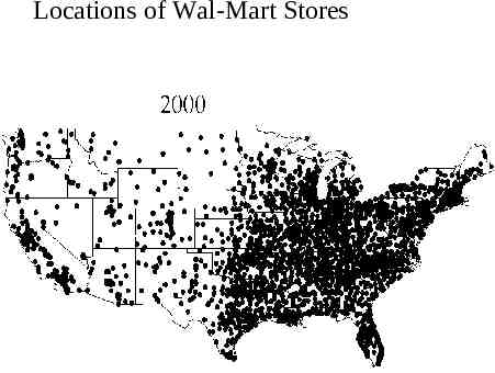
Identification “We figured we had to build our stores so that our distribution centers, or warehouses, could take care of them, but also so those stores could be controlled. We wanted them within reach of our district managers, and of ourselves here in Bentonville, so we could get out there and look after them. Each store had to be within a day’s drive of a distribution center” (Walton, 1992, pp. 110-111). “When you move like we did from town to town in these mostly rural areas, word of mouth gets your message out to customers pretty quickly without much advertising. When we had seventy-five stores in Arkansas, seventy-five in Missouri, eighty in Oklahoma, whatever, people knew who we were, and everybody except the merchants who weren’t discounting looked forward to our coming to their town. By doing it this way, we usually could get by with distributing just one advertising circular a month instead of running a whole lot of newspaper advertising” (Walton, 1992, p. 111).

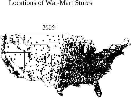
Locations of Wal-Mart Stores

Locations of Wal-Mart Stores

Locations of Wal-Mart Stores

Locations of Wal-Mart Stores

Locations of Wal-Mart Stores

Locations of Wal-Mart Stores

Locations of Wal-Mart Stores

Locations of Wal-Mart Stores

Locations of Wal-Mart Stores

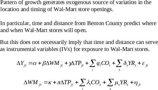
Pattern of growth generates exogenous source of variation in the location and timing of Wal-Mart store openings. In particular, time and distance from Benton County predict where and when Wal-Mart stores will open. But this does not necessarily imply that time and distance can serve as instrumental variables (IVs) for exposure to Wal-Mart stores. Y jt WM jt TPjt i COi sYRs jt i s WM jt TPjt i COs sYRs jt i s

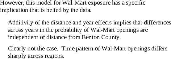
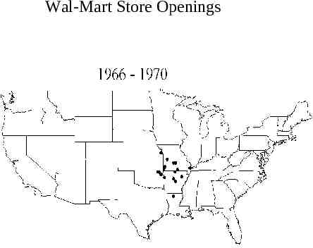
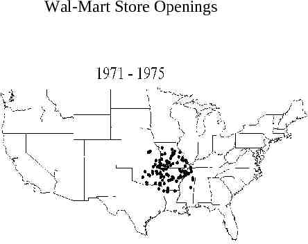
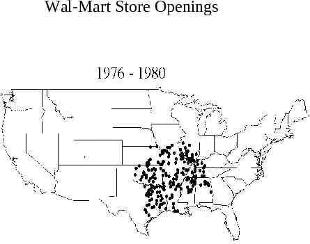
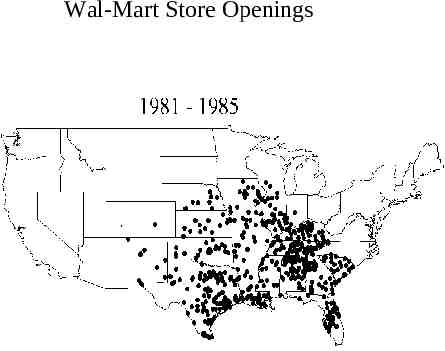
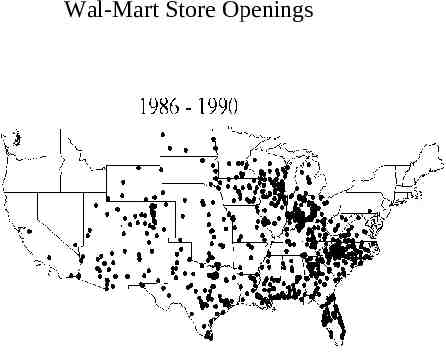
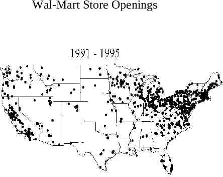
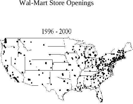
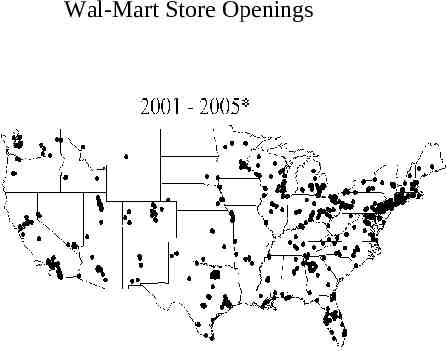
However, this model for Wal-Mart exposure has a specific implication that is belied by the data. Additivity of the distance and year effects implies that differences across years in the probability of Wal-Mart openings are independent of distance from Benton County. Clearly not the case. Time pattern of Wal-Mart openings differs sharply across regions.

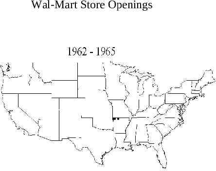
Wal-Mart Store Openings

Wal-Mart Store Openings

Wal-Mart Store Openings

Wal-Mart Store Openings

Wal-Mart Store Openings

Wal-Mart Store Openings

Wal-Mart Store Openings

Wal-Mart Store Openings

Wal-Mart Store Openings

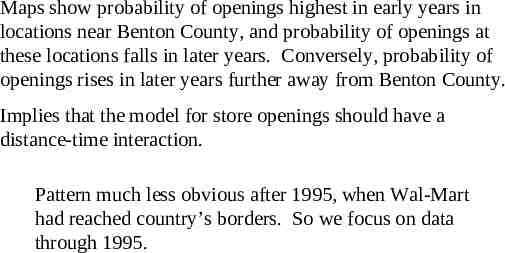
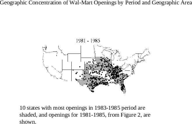
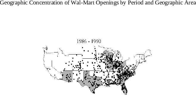
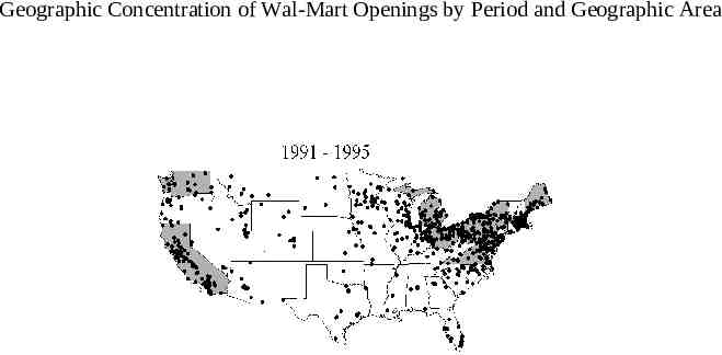
Maps show probability of openings highest in early years in locations near Benton County, and probability of openings at these locations falls in later years. Conversely, probability of openings rises in later years further away from Benton County. Implies that the model for store openings should have a distance-time interaction. Pattern much less obvious after 1995, when Wal-Mart had reached country’s borders. So we focus on data through 1995.

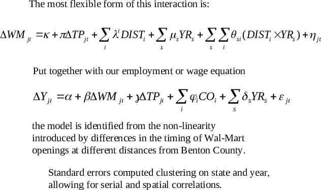
The most flexible form of this interaction is: WM jt TPjt i DISTi sYRs si ( DISTi YRs ) jt i s s i Put together with our employment or wage equation Y jt WM jt TPjt i COi sYRs jt i s the model is identified from the non-linearity introduced by differences in the timing of Wal-Mart openings at different distances from Benton County. Standard errors computed clustering on state and year, allowing for serial and spatial correlations.

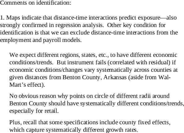
Comments on identification: 1. Maps indicate that distance-time interactions predict exposure—also strongly confirmed in regression analysis. Other key condition for identification is that we can exclude distance-time interactions from the employment and payroll models. We expect different regions, states, etc., to have different economic conditions/trends. But instrument fails (correlated with residual) if economic conditions/changes vary systematically across counties at given distances from Benton County, Arkansas (aside from WalMart’s effect). No obvious reason why points on circle of different radii around Benton County should have systematically different conditions/trends, especially for retail. Plus, recall that some specifications include county fixed effects, which capture systematically different growth rates.

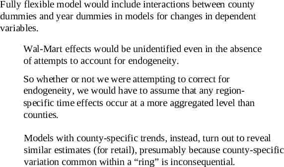
Fully flexible model would include interactions between county dummies and year dummies in models for changes in dependent variables. Wal-Mart effects would be unidentified even in the absence of attempts to account for endogeneity. So whether or not we were attempting to correct for endogeneity, we would have to assume that any regionspecific time effects occur at a more aggregated level than counties. Models with county-specific trends, instead, turn out to reveal similar estimates (for retail), presumably because county-specific variation common within a “ring” is inconsequential.

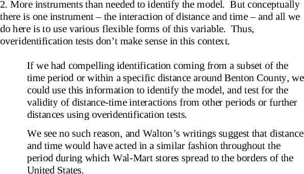
2. More instruments than needed to identify the model. But conceptually there is one instrument – the interaction of distance and time – and all we do here is to use various flexible forms of this variable. Thus, overidentification tests don’t make sense in this context. If we had compelling identification coming from a subset of the time period or within a specific distance around Benton County, we could use this information to identify the model, and test for the validity of distance-time interactions from other periods or further distances using overidentification tests. We see no such reason, and Walton’s writings suggest that distance and time would have acted in a similar fashion throughout the period during which Wal-Mart stores spread to the borders of the United States.

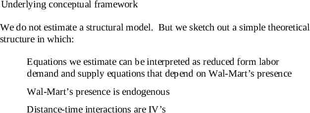
Underlying conceptual framework We do not estimate a structural model. But we sketch out a simple theoretical structure in which: Equations we estimate can be interpreted as reduced form labor demand and supply equations that depend on Wal-Mart’s presence Wal-Mart’s presence is endogenous Distance-time interactions are IV’s

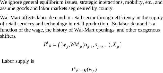
We ignore general equilibrium issues, strategic interactions, mobility, etc., and assume goods and labor markets segmented by county. Wal-Mart affects labor demand in retail sector through efficiency in the supply of retail services and technology in retail production. So labor demand is a function of the wage, the history of Wal-Mart openings, and other exogenous shifters. Ld jt f [ w jt ,WM jt (o jt 1 , o jt 2 ,.), X jt ] Labor supply is Ls jt g ( w jt )

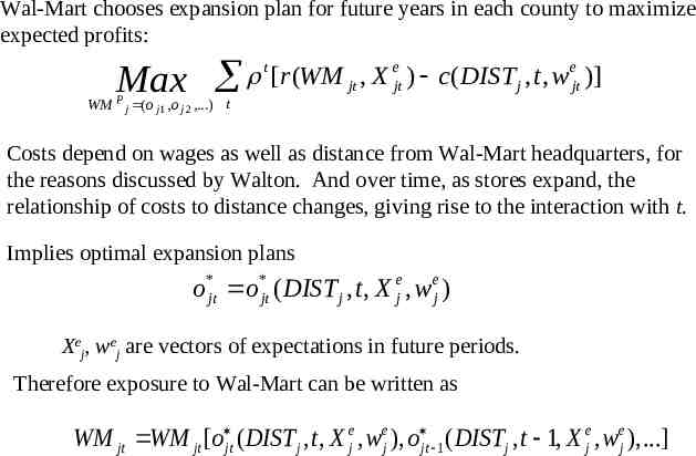
Wal-Mart chooses expansion plan for future years in each county to maximize expected profits: WM Max P j ( o j 1 , o j 2 ,.) t e e [ r ( WM , X ) c ( DIST , t , w jt jt j jt )] t Costs depend on wages as well as distance from Wal-Mart headquarters, for the reasons discussed by Walton. And over time, as stores expand, the relationship of costs to distance changes, giving rise to the interaction with t. Implies optimal expansion plans o*jt o*jt ( DIST j , t , X ej , wej ) Xej, wej are vectors of expectations in future periods. Therefore exposure to Wal-Mart can be written as WM jt WM jt [o jt ( DISTj , t , X ej , wej ), o jt 1 ( DISTj , t 1, X ej , wej ),.]

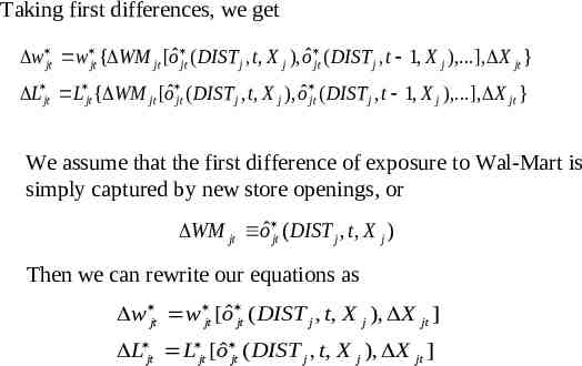
ô jt We substitute these into the labor demand equation in each period, obtaining Ld jt f {w jt ,WM jt [o jt ( DIST j , t , X ej , wej ), o jt 1 ( DIST j , t 1, X ej , wej ),.], X jt } Labor market equilibrium then gives w jt w jt {WM jt [oˆ jt ( DIST j , t , X j ), oˆ jt ( DIST j , t 1, X j ),.], X jt } L jt L jt {WM jt [oˆ jt ( DIST j , t , X j ), oˆ jt ( DIST j , t 1, X j ),.], X jt } ô jt is o jt evaluated at the equilibrium wage rates, i.e. oˆ jt ( DIST j , t , X j ) o jt ( DIST j , t , X j , w j )

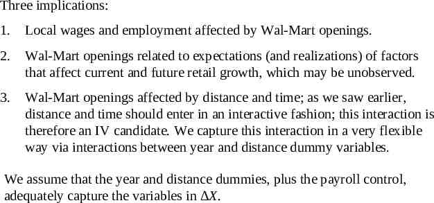
Taking first differences, we get w jt w jt { WM jt [oˆ jt ( DIST j , t , X j ), oˆ jt ( DIST j , t 1, X j ),.], X jt } L jt L jt { WM jt [oˆ jt ( DIST j , t , X j ), oˆ jt ( DIST j , t 1, X j ),.], X jt } We assume that the first difference of exposure to Wal-Mart is simply captured by new store openings, or WM jt oˆ jt ( DIST j , t , X j ) Then we can rewrite our equations as w jt w jt [oˆ jt ( DIST j , t , X j ), X jt ] L jt L jt [oˆ jt ( DIST j , t , X j ), X jt ]

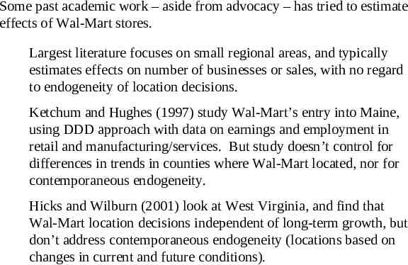
Three implications: 1. Local wages and employment affected by Wal-Mart openings. 2. Wal-Mart openings related to expectations (and realizations) of factors that affect current and future retail growth, which may be unobserved. 3. Wal-Mart openings affected by distance and time; as we saw earlier, distance and time should enter in an interactive fashion; this interaction is therefore an IV candidate. We capture this interaction in a very flexible way via interactions between year and distance dummy variables. We assume that the year and distance dummies, plus the payroll control, adequately capture the variables in X.

Some past academic work – aside from advocacy – has tried to estimate effects of Wal-Mart stores. Largest literature focuses on small regional areas, and typically estimates effects on number of businesses or sales, with no regard to endogeneity of location decisions. Ketchum and Hughes (1997) study Wal-Mart’s entry into Maine, using DDD approach with data on earnings and employment in retail and manufacturing/services. But study doesn’t control for differences in trends in counties where Wal-Mart located, nor for contemporaneous endogeneity. Hicks and Wilburn (2001) look at West Virginia, and find that Wal-Mart location decisions independent of long-term growth, but don’t address contemporaneous endogeneity (locations based on changes in current and future conditions).

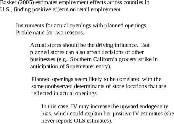
Basker (2005) estimates employment effects across counties in U.S., finding positive effects on retail employment. Instruments for actual openings with planned openings. Problematic for two reasons. Actual stores should be the driving influence. But planned stores can also affect decisions of other businesses (e.g., Southern California grocery strike in anticipation of Supercenter entry). Planned openings seem likely to be correlated with the same unobserved determinants of store locations that are reflected in actual openings. In this case, IV may increase the upward endogeneity bias, which could explain her positive IV estimates (she never reports OLS estimates).

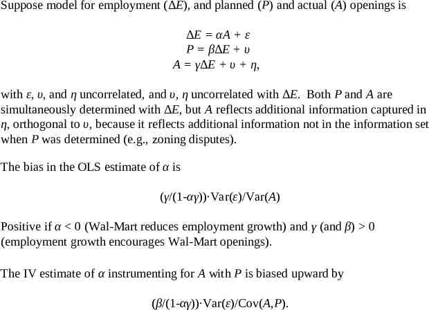
Suppose model for employment ( E), and planned (P) and actual (A) openings is E αA ε P β E υ A γ E υ η, with ε, υ, and η uncorrelated, and υ, η uncorrelated with E. Both P and A are simultaneously determined with E, but A reflects additional information captured in η, orthogonal to υ, because it reflects additional information not in the information set when P was determined (e.g., zoning disputes). The bias in the OLS estimate of α is (γ/(1-αγ)) Var(ε)/Var(A) Positive if α 0 (Wal-Mart reduces employment growth) and γ (and β) 0 (employment growth encourages Wal-Mart openings). The IV estimate of α instrumenting for A with P is biased upward by (β/(1-αγ)) Var(ε)/Cov(A,P).

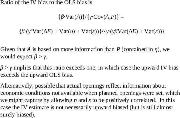
Ratio of the IV bias to the OLS bias is {β Var(A)}/{γ Cov(A,P)} {β (γ2Var( E) Var(υ) Var(ε))}/{γ (γβVar( E) Var(ε))} Given that A is based on more information than P (contained in η), we would expect β γ. β γ implies that this ratio exceeds one, in which case the upward IV bias exceeds the upward OLS bias. Alternatively, possible that actual openings reflect information about economic conditions not available when planned openings were set, which we might capture by allowing η and ε to be positively correlated. In this case the IV estimate is not necessarily upward biased (but is still almost surely biased).

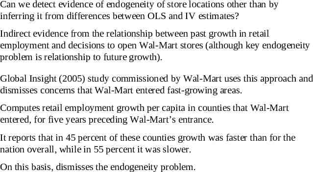
Can we detect evidence of endogeneity of store locations other than by inferring it from differences between OLS and IV estimates? Indirect evidence from the relationship between past growth in retail employment and decisions to open Wal-Mart stores (although key endogeneity problem is relationship to future growth). Global Insight (2005) study commissioned by Wal-Mart uses this approach and dismisses concerns that Wal-Mart entered fast-growing areas. Computes retail employment growth per capita in counties that Wal-Mart entered, for five years preceding Wal-Mart’s entrance. It reports that in 45 percent of these counties growth was faster than for the nation overall, while in 55 percent it was slower. On this basis, dismisses the endogeneity problem.

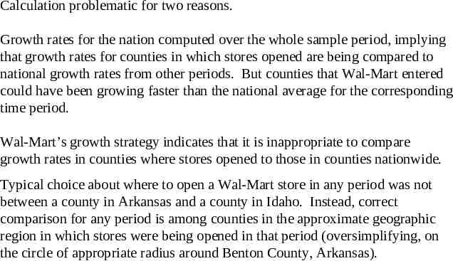
Calculation problematic for two reasons. Growth rates for the nation computed over the whole sample period, implying that growth rates for counties in which stores opened are being compared to national growth rates from other periods. But counties that Wal-Mart entered could have been growing faster than the national average for the corresponding time period. Wal-Mart’s growth strategy indicates that it is inappropriate to compare growth rates in counties where stores opened to those in counties nationwide. Typical choice about where to open a Wal-Mart store in any period was not between a county in Arkansas and a county in Idaho. Instead, correct comparison for any period is among counties in the approximate geographic region in which stores were being opened in that period (oversimplifying, on the circle of appropriate radius around Benton County, Arkansas).

Geographic Concentration of Wal-Mart Openings by Period and Geographic Area 10 states with most openings in 1983-1985 period are shaded, and openings for 1981-1985, from Figure 2, are shown.

Geographic Concentration of Wal-Mart Openings by Period and Geographic Area

Geographic Concentration of Wal-Mart Openings by Period and Geographic Area

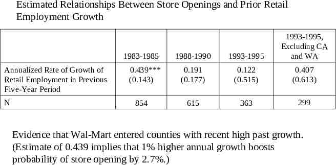
Estimated Relationships Between Store Openings and Prior Retail Employment Growth 1983-1985 Annualized Rate of Growth of Retail Employment in Previous Five-Year Period N 0.439*** (0.143) 854 1988-1990 1993-1995 1993-1995, Excluding CA and WA 0.191 (0.177) 0.122 (0.515) 0.407 (0.613) 615 363 299 Evidence that Wal-Mart entered counties with recent high past growth. (Estimate of 0.439 implies that 1% higher annual growth boosts probability of store opening by 2.7%.)

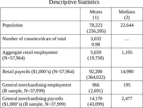
Descriptive Statistics Means (1) Medians (2) 78,223 (256,595) 22,644 3,032 0.98 . Aggregate retail employment (N 57,964) 5,659 (19,758) 1,105 Retail payrolls ( 1,000’s) (N 57,964) 92,208 (364,022) 14,990 General merchandising employment (B sample, N 37,999) 966 (2,691) 195 General merchandising payrolls ( 1,000’s) (B sample, N 37,999) 14,170 (43,099) 2,477 Population Number of counties/share of total

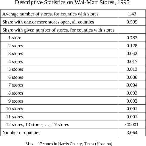
Descriptive Statistics on Wal-Mart Stores, 1995 Average number of stores, for counties with stores 1.43 Share with one or more stores open, all counties 0.505 Share with given number of stores, for counties with stores 1 store 0.783 2 stores 0.128 3 stores 0.042 4 stores 0.017 5 stores 0.013 6 stores 0.006 7 stores 0.004 8 stores 0.003 9 stores 0.002 10 stores 0.001 11 stores 0.001 12 stores, 13 stores, , 17 stores 0.001 Number of counties Max 17 stores in Harris County, Texas (Houston) 3,064

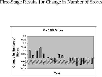
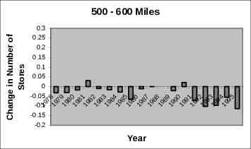
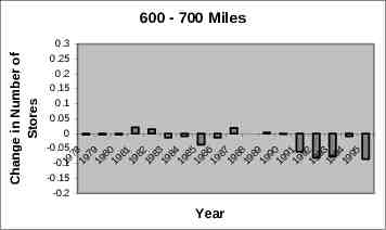
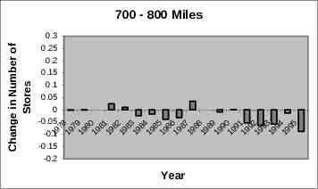
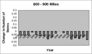
First-Stage Results for Change in Number of Stores 0 - 100 Miles Change in Number of Stores 0.3 0.25 0.2 0.15 0.1 0.05 0 -0.05 78 79 80 81 82 83 84 85 86 87 88 89 90 91 92 93 94 95 19 19 19 19 19 19 19 19 19 19 19 19 19 19 19 19 19 19 -0.1 -0.15 Year

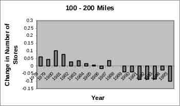
19 7 19 8 7 19 9 8 19 0 8 19 1 8 19 2 8 19 3 8 19 4 8 19 5 8 19 6 8 19 7 8 19 8 8 19 9 9 19 0 9 19 1 9 19 2 9 19 3 9 19 4 95 Change in Number of Stores 100 - 200 Miles 0.3 0.25 0.15 0.2 0.1 0.05 0 -0.05 -0.15 -0.1 Year

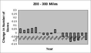
200 - 300 Miles Change in Number of Stores 0.3 0.25 0.2 0.15 0.1 0.05 0 -0.05 78 79 80 81 82 83 84 85 86 87 88 89 90 91 92 93 94 95 9 9 9 9 9 9 9 9 9 9 9 9 9 9 9 9 9 9 -0.11 1 1 1 1 1 1 1 1 1 1 1 1 1 1 1 1 1 -0.15 Year

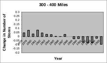
Change in Number of Stores 300 - 400 Miles 0.3 0.25 0.2 0.15 0.1 0.05 0 -0.05 8 9 0 1 2 3 4 5 6 7 8 9 0 1 2 3 4 5 7 7 8 8 8 8 8 8 8 8 8 8 9 9 9 9 9 9 -0.119 19 19 19 19 19 19 19 19 19 19 19 19 19 19 19 19 19 -0.15 -0.2 Year

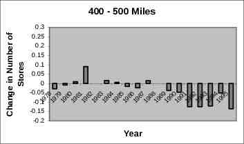
Change in Number of Stores 400 - 500 Miles 0.3 0.25 0.2 0.15 0.1 0.05 0 -0.05 8 9 0 1 2 3 4 5 6 7 8 9 0 1 2 3 4 5 7 7 8 8 8 8 8 8 8 8 8 8 9 9 9 9 9 9 -0.119 19 19 19 19 19 19 19 19 19 19 19 19 19 19 19 19 19 -0.15 -0.2 Year

Change in Number of Stores 0.3 0.25 0.2 0.15 0.1 0.05 0 -0.05 -0.1 -0.15 -0.2 19 78 19 79 19 80 19 81 19 82 19 83 19 84 19 85 19 86 19 87 19 88 19 89 19 90 19 91 19 9 19 2 93 19 9 19 4 95 500 - 600 Miles Year

Change in Number of Stores 600 - 700 Miles 0.3 0.25 0.2 0.15 0.1 0.05 0 -0.05 8 9 0 1 2 3 4 5 6 7 8 9 0 1 2 3 4 5 7 7 8 8 8 8 8 8 8 8 8 8 9 9 9 9 9 9 -0.119 19 19 19 19 19 19 19 19 19 19 19 19 19 19 19 19 19 -0.15 -0.2 Year

Change in Number of Stores 700 - 800 Miles 0.3 0.25 0.2 0.15 0.1 0.05 0 -0.05 8 9 0 1 2 3 4 5 6 7 8 9 0 1 2 3 4 5 7 7 8 8 8 8 8 8 8 8 8 8 9 9 9 9 9 9 -0.119 19 19 19 19 19 19 19 19 19 19 19 19 19 19 19 19 19 -0.15 -0.2 Year

Change in Number of Stores 800 - 900 Miles 0.3 0.25 0.2 0.15 0.1 0.05 0 -0.05 8 9 0 1 2 3 4 5 6 7 8 9 0 1 2 3 4 5 7 7 8 8 8 8 8 8 8 8 8 8 9 9 9 9 9 9 -0.119 19 19 19 19 19 19 19 19 19 19 19 19 19 19 19 19 19 -0.15 -0.2 Year

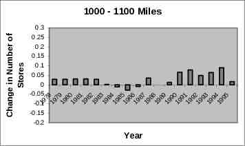
Change in Number of Stores 1000 - 1100 Miles 0.3 0.25 0.2 0.15 0.1 0.05 0 -0.05 8 9 0 1 2 3 4 5 6 7 8 9 0 1 2 3 4 5 7 7 8 8 8 8 8 8 8 8 8 8 9 9 9 9 9 9 -0.119 19 19 19 19 19 19 19 19 19 19 19 19 19 19 19 19 19 -0.15 -0.2 Year

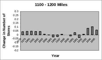
Change in Number of Stores 1100 - 1200 Miles 0.3 0.25 0.2 0.15 0.1 0.05 0 -0.05 8 9 0 1 2 3 4 5 6 7 8 9 0 1 2 3 4 5 7 7 8 8 8 8 8 8 8 8 8 8 9 9 9 9 9 9 -0.119 19 19 19 19 19 19 19 19 19 19 19 19 19 19 19 19 19 -0.15 -0.2 Year

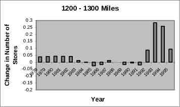
Change in Number of Stores 1200 - 1300 Miles 0.3 0.25 0.2 0.15 0.1 0.05 0 -0.05 8 9 0 1 2 3 4 5 6 7 8 9 0 1 2 3 4 5 7 7 8 8 8 8 8 8 8 8 8 8 9 9 9 9 9 9 -0.119 19 19 19 19 19 19 19 19 19 19 19 19 19 19 19 19 19 -0.15 -0.2 Year

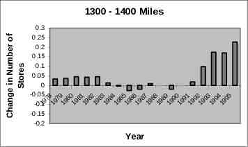
Change in Number of Stores 1300 - 1400 Miles 0.3 0.25 0.2 0.15 0.1 0.05 0 -0.05 8 9 0 1 2 3 4 5 6 7 8 9 0 1 2 3 4 5 7 7 8 8 8 8 8 8 8 8 8 8 9 9 9 9 9 9 -0.119 19 19 19 19 19 19 19 19 19 19 19 19 19 19 19 19 19 -0.15 -0.2 Year

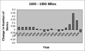
Change in Number of Stores 1400 - 1500 Miles 0.3 0.25 0.2 0.15 0.1 0.05 0 -0.05 8 9 0 1 2 3 4 5 6 7 8 9 0 1 2 3 4 5 7 7 8 8 8 8 8 8 8 8 8 8 9 9 9 9 9 9 -0.119 19 19 19 19 19 19 19 19 19 19 19 19 19 19 19 19 19 -0.15 -0.2 Year

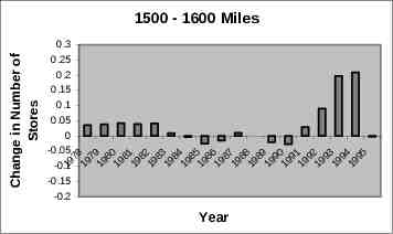
Change in Number of Stores 1500 - 1600 Miles 0.3 0.25 0.2 0.15 0.1 0.05 0 -0.05 8 9 0 1 2 3 4 5 6 7 8 9 0 1 2 3 4 5 7 7 8 8 8 8 8 8 8 8 8 8 9 9 9 9 9 9 -0.119 19 19 19 19 19 19 19 19 19 19 19 19 19 19 19 19 19 -0.15 -0.2 Year

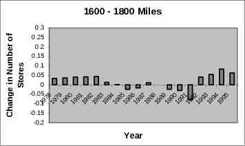
Change in Number of Stores 1600 - 1800 Miles 0.3 0.25 0.2 0.15 0.1 0.05 0 -0.05 8 9 0 1 2 3 4 5 6 7 8 9 0 1 2 3 4 5 7 7 8 8 8 8 8 8 8 8 8 8 9 9 9 9 9 9 -0.119 19 19 19 19 19 19 19 19 19 19 19 19 19 19 19 19 19 -0.15 -0.2 Year

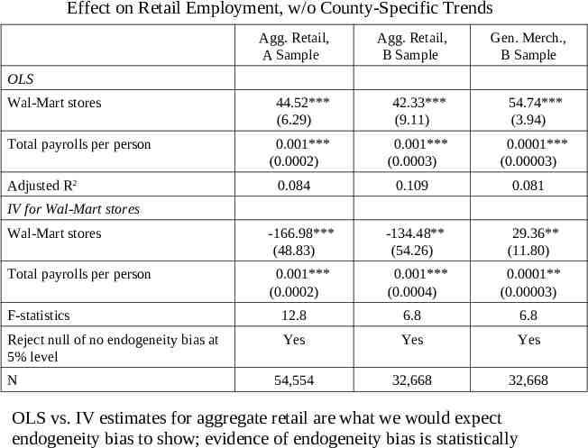
Effect on Retail Employment, w/o County-Specific Trends Agg. Retail, A Sample Agg. Retail, B Sample Gen. Merch., B Sample 44.52*** (6.29) 42.33*** (9.11) 54.74*** (3.94) 0.001*** (0.0002) 0.001*** (0.0003) 0.0001*** (0.00003) OLS Wal-Mart stores Total payrolls per person Adjusted R2 0.084 0.109 0.081 IV for Wal-Mart stores Wal-Mart stores -166.98*** (48.83) -134.48** (54.26) 29.36** (11.80) Total payrolls per person 0.001*** (0.0002) 0.001*** (0.0004) 0.0001** (0.00003) F-statistics 12.8 6.8 6.8 Reject null of no endogeneity bias at 5% level Yes Yes Yes 54,554 32,668 32,668 N OLS vs. IV estimates for aggregate retail are what we would expect endogeneity bias to show; evidence of endogeneity bias is statistically

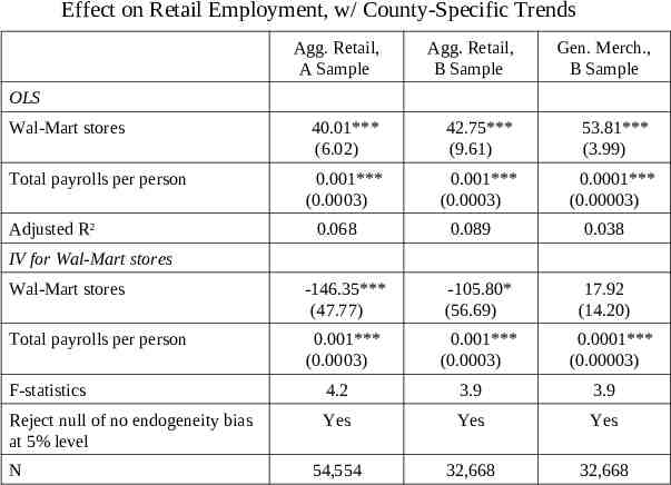
Effect on Retail Employment, w/ County-Specific Trends Agg. Retail, A Sample Agg. Retail, B Sample Gen. Merch., B Sample 40.01*** (6.02) 42.75*** (9.61) 53.81*** (3.99) 0.001*** (0.0003) 0.001*** (0.0003) 0.0001*** (0.00003) OLS Wal-Mart stores Total payrolls per person Adjusted R2 0.068 0.089 0.038 IV for Wal-Mart stores Wal-Mart stores -146.35*** (47.77) -105.80* (56.69) Total payrolls per person 0.001*** (0.0003) 0.001*** (0.0003) 17.92 (14.20) 0.0001*** (0.00003) F-statistics 4.2 3.9 3.9 Reject null of no endogeneity bias at 5% level Yes Yes Yes 54,554 32,668 32,668 N

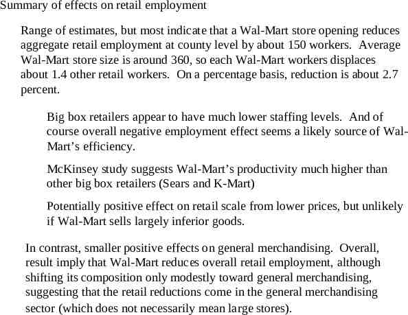
Summary of effects on retail employment Range of estimates, but most indicate that a Wal-Mart store opening reduces aggregate retail employment at county level by about 150 workers. Average Wal-Mart store size is around 360, so each Wal-Mart workers displaces about 1.4 other retail workers. On a percentage basis, reduction is about 2.7 percent. Big box retailers appear to have much lower staffing levels. And of course overall negative employment effect seems a likely source of WalMart’s efficiency. McKinsey study suggests Wal-Mart’s productivity much higher than other big box retailers (Sears and K-Mart) Potentially positive effect on retail scale from lower prices, but unlikely if Wal-Mart sells largely inferior goods. In contrast, smaller positive effects on general merchandising. Overall, result imply that Wal-Mart reduces overall retail employment, although shifting its composition only modestly toward general merchandising, suggesting that the retail reductions come in the general merchandising sector (which does not necessarily mean large stores).

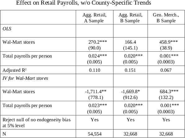
Effect on Retail Payrolls, w/o County-Specific Trends Agg. Retail, A Sample Agg. Retail, B Sample Gen. Merch., B Sample OLS Wal-Mart stores 270.2*** (90.0) 166.4 (145.1) Total payrolls per person 0.024*** (0.005) 0.020*** (0.005) Adjusted R2 0.110 0.151 -1,711.4** (778.1) -1,669.8* (912.6) 458.9*** (38.9) 0.001*** (0.0003) 0.067 IV for Wal-Mart stores Wal-Mart stores Total payrolls per person Reject null of no endogeneity bias at 5% level N 0.023*** (0.005) 0.020*** (0.005) 684.3*** (132.2) 0.001*** (0.0003) Yes Yes Yes 54,554 32,668 32,668

Effect on Retail Payrolls, w/ County-Specific Trends Agg. Retail, A Sample Agg. Retail, B Sample Gen. Merch., B Sample OLS Wal-Mart stores 233.1*** (89.7) 172.5 (154.1) Total payrolls per person 0.023*** (0.005) 0.020*** (0.006) Adjusted R2 0.094 0.123 427.6*** (39.3) 0.002*** (0.0003) 0.039 IV for Wal-Mart stores Wal-Mart stores -1,149.8 (735.8) -1,547.6* (894.4) 525.4*** (149.2) Total payrolls per person 0.023*** (0.005) 0.020*** (0.006) 0.002*** (0.0003) Reject null of no endogeneity bias at 5% level N Yes Yes No 54,554 32,668 32,668

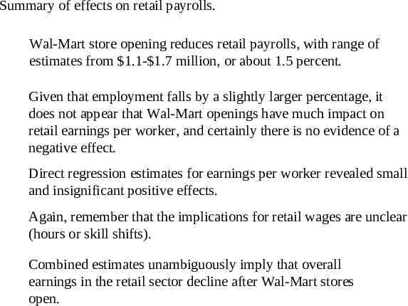
Summary of effects on retail payrolls. Wal-Mart store opening reduces retail payrolls, with range of estimates from 1.1- 1.7 million, or about 1.5 percent. Given that employment falls by a slightly larger percentage, it does not appear that Wal-Mart openings have much impact on retail earnings per worker, and certainly there is no evidence of a negative effect. Direct regression estimates for earnings per worker revealed small and insignificant positive effects. Again, remember that the implications for retail wages are unclear (hours or skill shifts). Combined estimates unambiguously imply that overall earnings in the retail sector decline after Wal-Mart stores open.

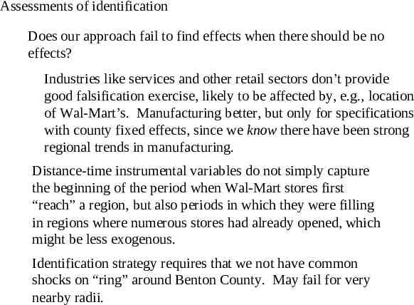
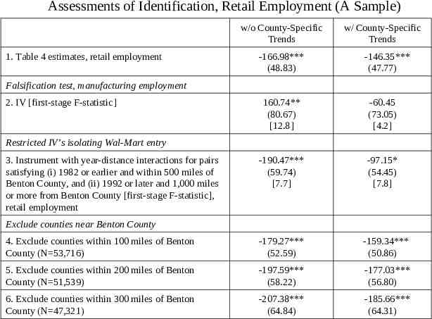
Assessments of identification Does our approach fail to find effects when there should be no effects? Industries like services and other retail sectors don’t provide good falsification exercise, likely to be affected by, e.g., location of Wal-Mart’s. Manufacturing better, but only for specifications with county fixed effects, since we know there have been strong regional trends in manufacturing. Distance-time instrumental variables do not simply capture the beginning of the period when Wal-Mart stores first “reach” a region, but also periods in which they were filling in regions where numerous stores had already opened, which might be less exogenous. Identification strategy requires that we not have common shocks on “ring” around Benton County. May fail for very nearby radii.

Assessments of Identification, Retail Employment (A Sample) w/o County-Specific Trends 1. Table 4 estimates, retail employment -166.98*** (48.83) w/ County-Specific Trends -146.35*** (47.77) Falsification test, manufacturing employment 2. IV [first-stage F-statistic] 160.74** (80.67) [12.8] -60.45 (73.05) [4.2] -190.47*** (59.74) [7.7] -97.15* (54.45) [7.8] Restricted IV’s isolating Wal-Mart entry 3. Instrument with year-distance interactions for pairs satisfying (i) 1982 or earlier and within 500 miles of Benton County, and (ii) 1992 or later and 1,000 miles or more from Benton County [first-stage F-statistic], retail employment Exclude counties near Benton County 4. Exclude counties within 100 miles of Benton County (N 53,716) -179.27*** (52.59) -159.34*** (50.86) 5. Exclude counties within 200 miles of Benton County (N 51,539) -197.59*** (58.22) -177.03*** (56.80) 6. Exclude counties within 300 miles of Benton County (N 47,321) -207.38*** (64.84) -185.66*** (64.31)

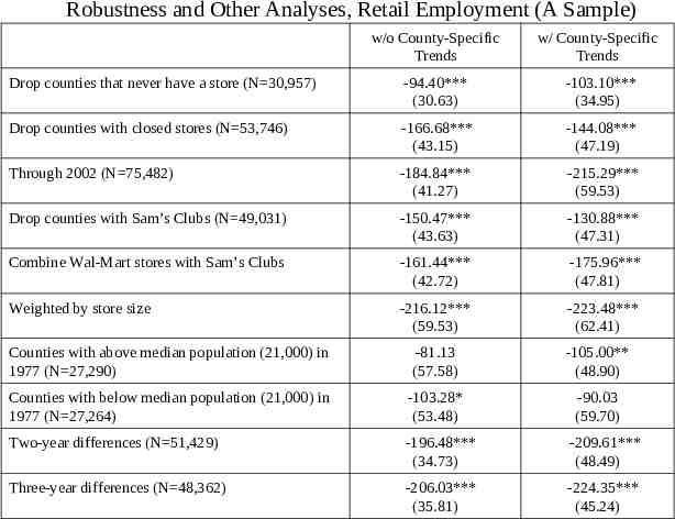
Robustness and Other Analyses, Retail Employment (A Sample) w/o County-Specific Trends w/ County-Specific Trends Drop counties that never have a store (N 30,957) -94.40*** (30.63) -103.10*** (34.95) Drop counties with closed stores (N 53,746) -166.68*** (43.15) -144.08*** (47.19) Through 2002 (N 75,482) -184.84*** (41.27) -215.29*** (59.53) Drop counties with Sam’s Clubs (N 49,031) -150.47*** (43.63) -130.88*** (47.31) Combine Wal-Mart stores with Sam’s Clubs -161.44*** (42.72) -175.96*** (47.81) Weighted by store size -216.12*** (59.53) -223.48*** (62.41) Counties with above median population (21,000) in 1977 (N 27,290) -81.13 (57.58) -105.00** (48.90) Counties with below median population (21,000) in 1977 (N 27,264) -103.28* (53.48) -90.03 (59.70) Two-year differences (N 51,429) -196.48*** (34.73) -209.61*** (48.49) Three-year differences (N 48,362) -206.03*** (35.81) -224.35*** (45.24)

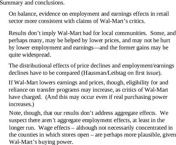
Summary and conclusions. On balance, evidence on employment and earnings effects in retail sector more consistent with claims of Wal-Mart’s critics. Results don’t imply Wal-Mart bad for local communities. Some, and perhaps many, may be helped by lower prices, and may not be hurt by lower employment and earnings—and the former gains may be quite widespread. The distributional effects of price declines and employment/earnings declines have to be compared (Hausman/Leibtag on first issue). If Wal-Mart lowers earnings and prices, though, eligibility for and reliance on transfer programs may increase, as critics of Wal-Mart have charged. (And this may occur even if real purchasing power increases.) Note, though, that our results don’t address aggregate effects. We suspect there aren’t aggregate employment effects, at least in the longer run. Wage effects – although not necessarily concentrated in the counties in which stores open – are perhaps more plausible, given Wal-Mart’s buying power.