TAG: A Tiny Aggregation Service for Ad-Hoc Sensor Networks Samuel

TAG: A Tiny Aggregation Service for Ad-Hoc Sensor Networks Samuel Madden UC Berkeley with Michael Franklin, Joseph Hellerstein, and Wei Hong December 9th, 2002 @ OSDI 1

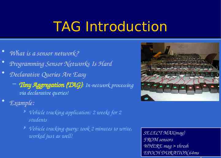
TAG Introduction What is a sensor network? Programming Sensor Networks Is Hard Declarative Queries Are Easy – Tiny Aggregation (TAG): In-network processing via declarative queries! Example: » Vehicle tracking application: 2 weeks for 2 students » Vehicle tracking query: took 2 minutes to write, worked just as well! SELECT MAX(mag) FROM sensors WHERE mag thresh EPOCH DURATION 64ms 2

Overview Sensor Networks Queries in Sensor Nets Tiny Aggregation – Overview – Simulation & Results 3

Overview Sensor Networks Queries in Sensor Nets Tiny Aggregation – Overview – Simulation & Results 4

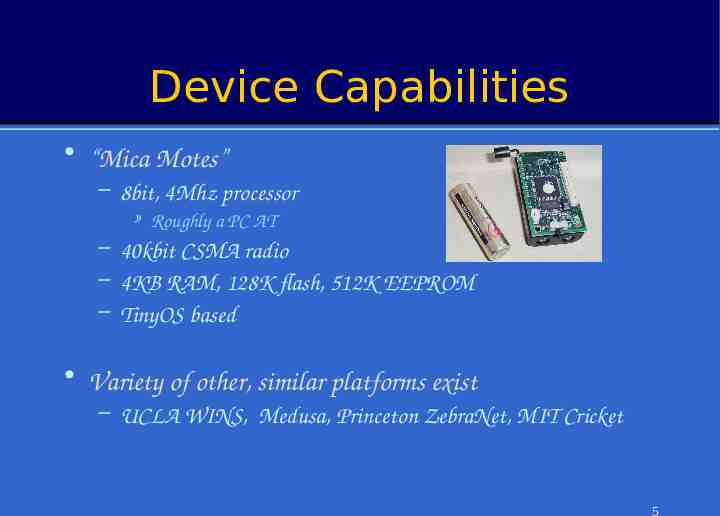
Device Capabilities “Mica Motes” – 8bit, 4Mhz processor » Roughly a PC AT – 40kbit CSMA radio – 4KB RAM, 128K flash, 512K EEPROM – TinyOS based Variety of other, similar platforms exist – UCLA WINS, Medusa, Princeton ZebraNet, MIT Cricket 5

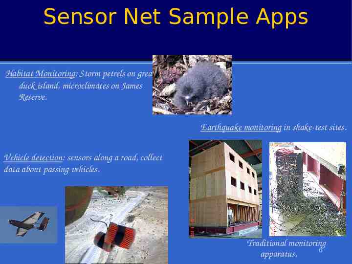
Sensor Net Sample Apps Habitat Monitoring: Storm petrels on great duck island, microclimates on James Reserve. Earthquake monitoring in shake-test sites. Vehicle detection: sensors along a road, collect data about passing vehicles. Traditional monitoring 6 apparatus.

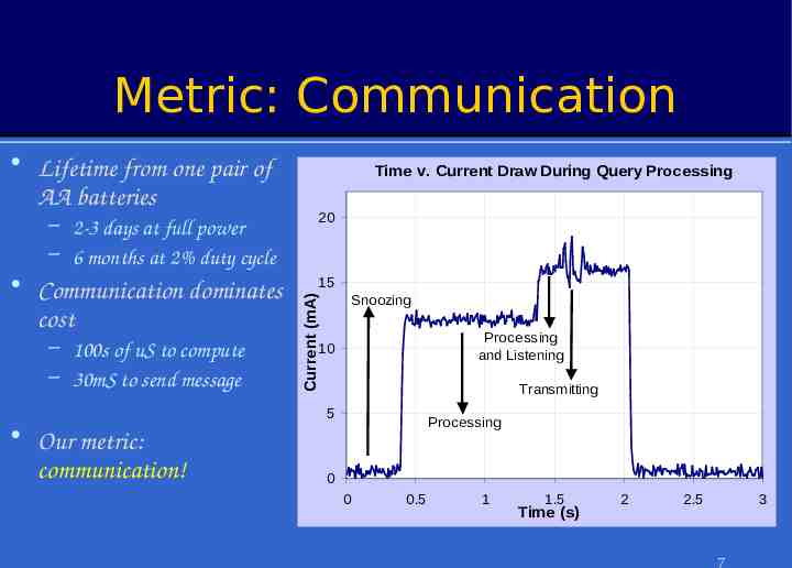
Metric: Communication – 2-3 days at full power – 6 months at 2% duty cycle Communication dominates cost – 100s of uS to compute – 30mS to send message Time v. Current Draw During Query Processing 20 15 Snoozing Current (mA) Lifetime from one pair of AA batteries Processing and Listening 10 Transmitting 5 Our metric: communication! Processing 0 0 0.5 1 1.5 Time (s) 2 2.5 3 7

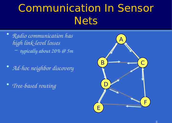
Communication In Sensor Nets Radio communication has high link-level losses A – typically about 20% @ 5m B Ad-hoc neighbor discovery C D Tree-based routing E F 8

Overview Sensor Networks Queries in Sensor Nets Tiny Aggregation – Overview – Optimizations & Results 9

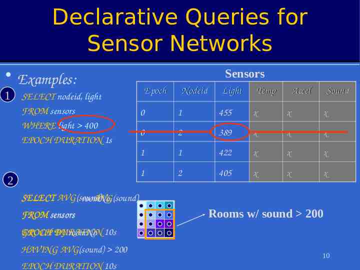
Declarative Queries for Sensor Networks Examples: 1 SELECT nodeid, light FROM sensors WHERE light 400 EPOCH DURATION 1s 2 Sensors Epoch Nodeid Light Temp Accel Sound 0 1 455 x x x 0 2 389 x x x 1 1 422 x x x 1 2 405 x x x SELECT AVG(sound) AVG(sound) roomNo, FROM sensors Rooms w/ sound 200 EPOCH DURATION GROUP BY roomNo 10s HAVING AVG(sound) 200 EPOCH DURATION 10s 10

Overview Sensor Networks Queries in Sensor Nets Tiny Aggregation – Overview – Optimizations & Results 11

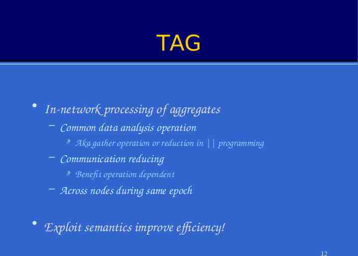
TAG In-network processing of aggregates – Common data analysis operation » Aka gather operation or reduction in programming – Communication reducing » Benefit operation dependent – Across nodes during same epoch Exploit semantics improve efficiency! 12

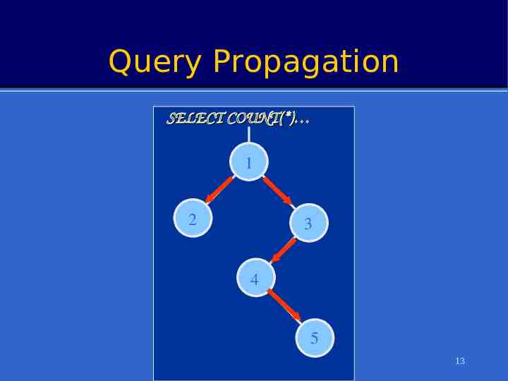
Query Propagation SELECT COUNT(*) 1 2 3 4 5 13

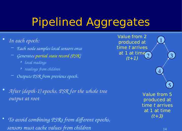
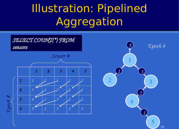
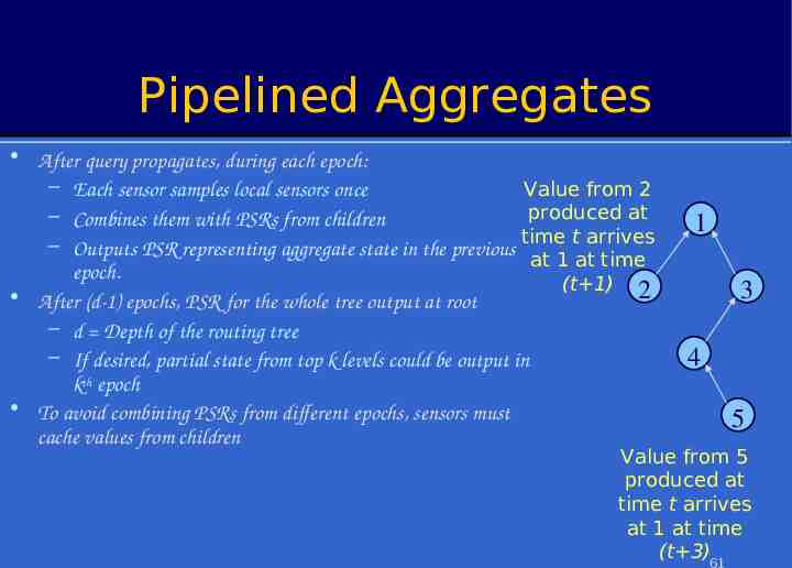
Pipelined Aggregates In each epoch: – Each node samples local sensors once – Generates partial state record (PSR) » local readings » readings from children – Outputs PSR from previous epoch. After (depth-1) epochs, PSR for the whole tree output at root To avoid combining PSRs from different epochs, sensors must cache values from children Value from 2 produced at time t arrives at 1 at time 2 (t 1) 1 3 4 5 Value from 5 produced at time t arrives at 1 at time (t 3) 14

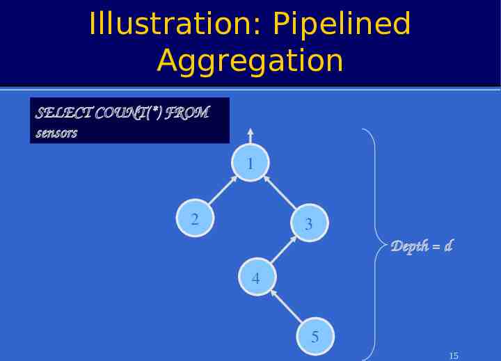
Illustration: Pipelined Aggregation SELECT COUNT(*) FROM sensors 1 2 3 Depth d 4 5 15

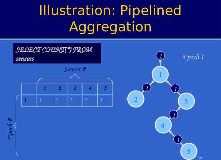
Illustration: Pipelined Aggregation SELECT COUNT(*) FROM sensors Sensor # 1 Epoch # 1 1 2 1 3 1 1 1 4 1 Epoch 1 1 5 1 1 2 3 1 4 1 5 16

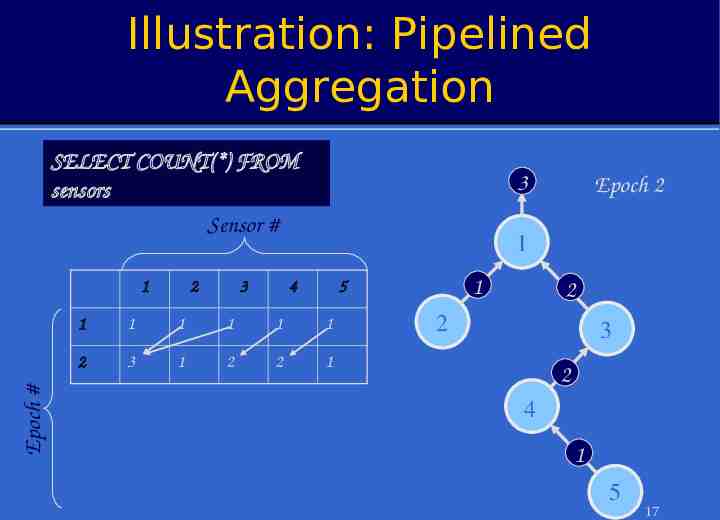
Illustration: Pipelined Aggregation SELECT COUNT(*) FROM sensors Sensor # Epoch # 1 2 3 3 Epoch 2 1 4 1 5 1 1 1 1 1 1 2 3 1 2 2 1 2 2 3 2 4 1 5 17

Illustration: Pipelined Aggregation SELECT COUNT(*) FROM sensors Sensor # Epoch # 1 2 3 4 Epoch 3 1 4 1 5 1 1 1 1 1 1 2 3 1 2 2 1 3 4 1 3 2 1 3 2 3 2 4 1 5 18

Illustration: Pipelined Aggregation SELECT COUNT(*) FROM sensors Sensor # Epoch # 1 2 3 5 Epoch 4 1 4 1 5 1 1 1 1 1 1 2 3 1 2 2 1 3 4 1 3 2 1 4 5 1 3 2 1 3 2 3 2 4 1 5 19

Illustration: Pipelined Aggregation SELECT COUNT(*) FROM sensors Sensor # Epoch # 1 2 3 5 Epoch 5 1 4 1 5 1 1 1 1 1 1 2 3 1 2 2 1 3 4 1 3 2 1 4 5 1 3 2 1 5 5 1 3 2 1 3 2 3 2 4 1 5 20

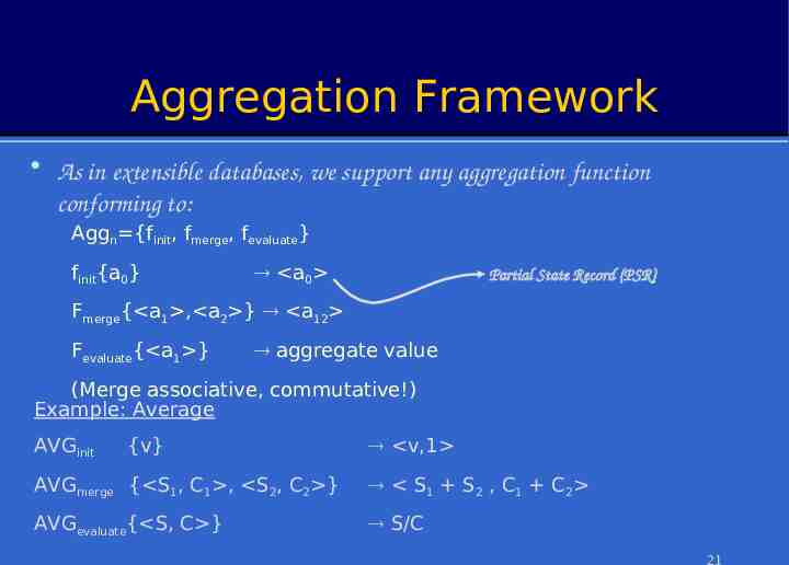
Aggregation Framework As in extensible databases, we support any aggregation function conforming to: Aggn {finit, fmerge, fevaluate} finit{a0} a0 Partial State Record (PSR) Fmerge{ a1 , a2 } a12 Fevaluate{ a1 } aggregate value (Merge associative, commutative!) Example: Average AVGinit {v} v,1 AVGmerge { S1, C1 , S2, C2 } S1 S2 , C1 C2 AVGevaluate{ S, C } S/C 21

Types of Aggregates SQL supports MIN, MAX, SUM, COUNT, AVERAGE Any function can be computed via TAG In network benefit for many operations – E.g. Standard deviation, top/bottom N, spatial union/intersection, histograms, etc. – Compactness of PSR 22

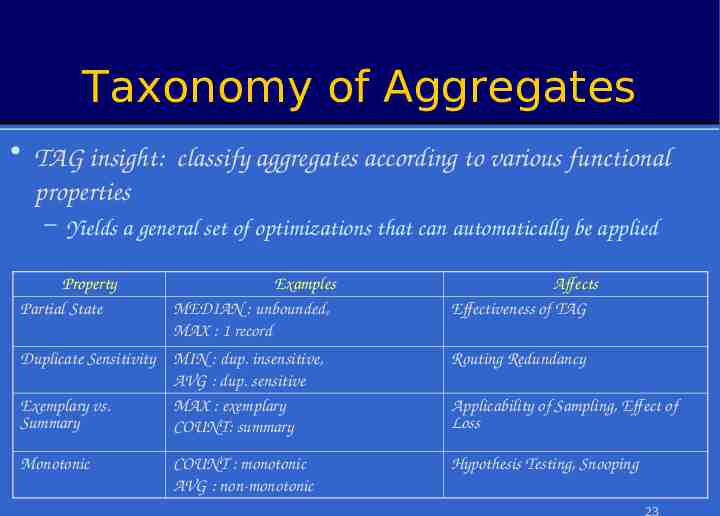
Taxonomy of Aggregates TAG insight: classify aggregates according to various functional properties – Yields a general set of optimizations that can automatically be applied Property Partial State Examples MEDIAN : unbounded, MAX : 1 record Affects Effectiveness of TAG Duplicate Sensitivity MIN : dup. insensitive, AVG : dup. sensitive Exemplary vs. MAX : exemplary Summary COUNT: summary Routing Redundancy Monotonic Hypothesis Testing, Snooping COUNT : monotonic AVG : non-monotonic Applicability of Sampling, Effect of Loss 23

TAG Advantages Communication Reduction – Important for power and contention Continuous stream of results – In the absence of faults, will converge to right answer Lots of optimizations – Based on shared radio channel – Semantics of operators 24

Simulation Environment Evaluated via simulation Coarse grained event based simulator – Sensors arranged on a grid – Two communication models » Lossless: All neighbors hear all messages » Lossy: Messages lost with probability that increases with distance 25

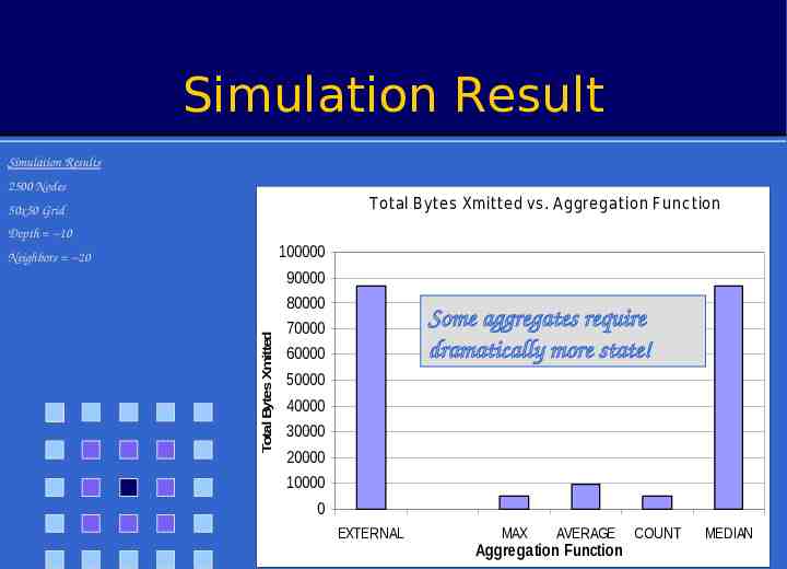
Simulation Result Simulation Results 2500 Nodes Total Bytes Xmitted vs. Aggregation Func tion 50x50 Grid Depth 10 100000 Neighbors 20 Total Bytes Xmitted 90000 80000 Some aggregates require dramatically more state! 70000 60000 50000 40000 30000 20000 10000 0 EXTERNAL MAX AVERAGE Aggregation Function COUNT MEDIAN 26

Optimization: Channel Sharing (“Snooping”) Insight: Shared channel enables optimizations Suppress messages that won’t affect aggregate – E.g., MAX – Applies to all exemplary, monotonic aggregates 27

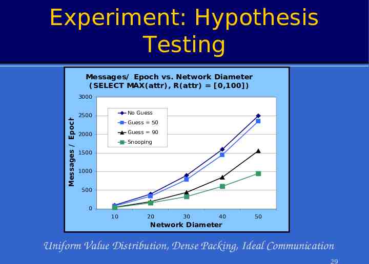
Optimization: Hypothesis Testing Insight: Guess from root can be used for suppression – E.g. ‘MIN 50’ – Works for monotonic & exemplary aggregates » Also summary, if imprecision allowed How is hypothesis computed? – Blind or statistically informed guess – Observation over network subset 28

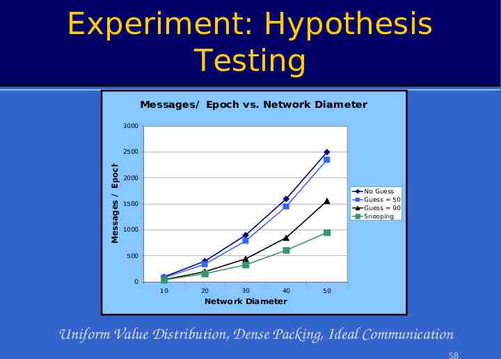
Experiment: Hypothesis Testing Messages/ Epoch vs. Network Diameter (SELECT MAX(attr), R(attr) [0,100]) Messages / Epoch 3000 No Guess 2500 Guess 50 Guess 90 2000 Snooping 1500 1000 500 0 10 20 30 40 50 Network Diameter Uniform Value Distribution, Dense Packing, Ideal Communication 29

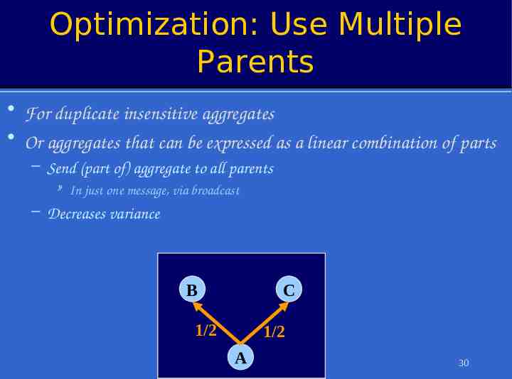
Optimization: Use Multiple Parents For duplicate insensitive aggregates Or aggregates that can be expressed as a linear combination of parts – Send (part of) aggregate to all parents » In just one message, via broadcast – Decreases variance B C 1/2 1 1/2 A 30

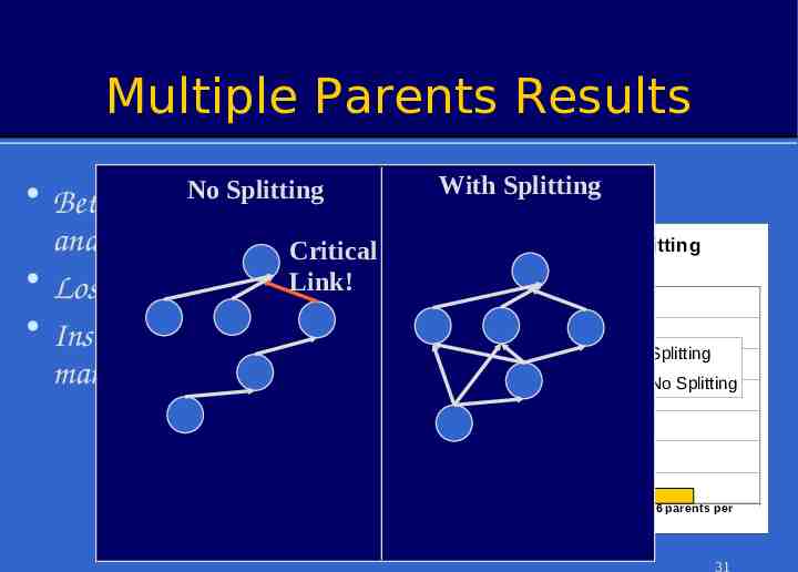
Multiple Parents Results With Splitting Benefit of Result Splitting (COUNT query) 1400 1200 Avg. COUNT Splitting Better thanNoprevious analysis expected! Critical Losses aren’t independent! Link! Insight: spreads data over many links 1000 800 Splitting No Splitting 600 400 200 0 (2500 nodes, lossy radio model, 6 parents per node) 31

Summary TAG enables in-network declarative query processing – State dependent communication benefit – Transparent optimization via taxonomy » Hypothesis Testing » Parent Sharing Declarative queries are the right interface for data collection in sensor nets! – Easier to program and more efficient for vast majority of users TinyDB Release Available - http://telegraph.cs.berkeley.edu/tinydb 32

Questions? TinyDB Demo After The Session 33

TinyOS Operating system from David Culler’s group at Berkeley C-like programming environment Provides messaging layer, abstractions for major hardware components – Split phase highly asynchronous, interrupt-driven programming model Hill, Szewczyk, Woo, Culler, & Pister. “Systems Architecture Directions for Networked Sensors.” 34 ASPLOS 2000. See http://webs.cs.berkeley.edu/tos

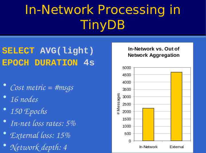
In-Network Processing in TinyDB SELECT AVG(light) EPOCH DURATION 4s In-Network vs. Out of Network Aggregation 5000 4500 3500 # Messages Cost metric #msgs 16 nodes 150 Epochs In-net loss rates: 5% External loss: 15% Network depth: 4 4000 3000 2500 2000 1500 1000 500 0 In-Network External 35

Grouping Recall: GROUP BY expression partitions sensors into distinct logical groups – E.g. “partition sensors by room number” If query is grouped, sensors apply expression on each epoch PSRs tagged with group When a PSR (with group) is received: – If it belongs to a stored group, merge with existing PSR – If not, just store it At the end of each epoch, transmit one PSR per group Need to evict if storage overflows. 36

Group Eviction Problem: Number of groups in any one iteration may exceed available storage on sensor Solution: Evict! (Partial Preaggregation*) – Choose one or more groups to forward up tree – Rely on nodes further up tree, or root, to recombine groups properly – What policy to choose? » Intuitively: least popular group, since don’t want to evict a group that will receive more values this epoch. » Experiments suggest: Policy matters very little Evicting as many groups as will fit into a single message is good 37 * Per-Åke Larson. Data Reduction by Partial Preaggregation. ICDE 2002.

Declarative Benefits In Sensor Networks Vastly simplifies execution for large networks – Since locations are described by predicates – Operations are over groups Enables tolerance to faults – Since system is free to choose where and when operations happen Data independence – System is free to choose where data lives, how it is represented 38

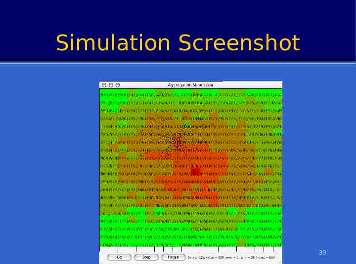
Simulation Screenshot 39

Hypothesis Testing For Average AVERAGE: each node suppresses readings within some of a approximate average µ*. – Parents assume children who don’t report have value µ* Computed average cannot be off by more than . 40

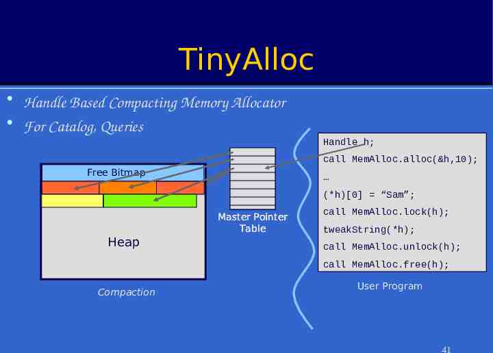
TinyAlloc Handle Based Compacting Memory Allocator For Catalog, Queries Handle h; call MemAlloc.alloc(&h,10); Free Bitmap (*h)[0] “Sam”; Master Pointer Table Heap call MemAlloc.lock(h); tweakString(*h); call MemAlloc.unlock(h); call MemAlloc.free(h); Compaction User Program 41

Schema Attribute & Command IF – At INIT(), components register attributes and commands they support » Commands implemented via wiring » Attributes fetched via accessor command – Catalog API allows local and remote queries over known attributes / commands. Demo of adding an attribute, executing a command. 42

Q1: Expressiveness Simple data collection satisfies most users How much of what people want to do is just simple aggregates? – Anecdotally, most of it – EE people want filters simple statistics (unless they can have signal processing) However, we’d like to satisfy everyone! 43

Query Language New Features: – Joins – Event-based triggers » Via extensible catalog – In network & nested queries – Split-phase (offline) delivery » Via buffers 44

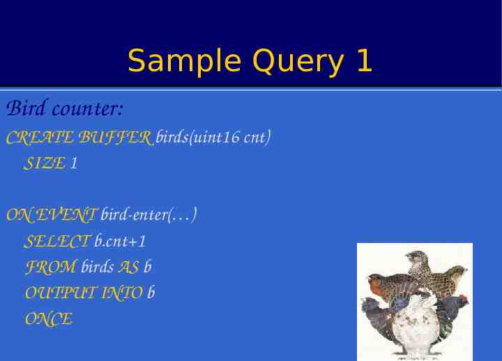
Sample Query 1 Bird counter: CREATE BUFFER birds(uint16 cnt) SIZE 1 ON EVENT bird-enter( ) SELECT b.cnt 1 FROM birds AS b OUTPUT INTO b ONCE 45

Sample Query 2 Birds that entered and left within time t of each other: ON EVENT bird-leave AND bird-enter WITHIN t SELECT bird-leave.time, bird-leave.nest WHERE bird-leave.nest bird-enter.nest ONCE 46

Sample Query 3 Delta compression: SELECT light FROM buf, sensors WHERE s.light – buf.light t OUTPUT INTO buf SAMPLE PERIOD 1s 47

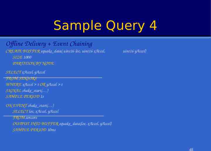
Sample Query 4 Offline Delivery Event Chaining CREATE BUFFER equake data( uint16 loc, uint16 xAccel, SIZE 1000 PARTITION BY NODE uint16 yAccel) SELECT xAccel, yAccel FROM SENSORS WHERE xAccel t OR yAccel t SIGNAL shake start( ) SAMPLE PERIOD 1s ON EVENT shake start( ) SELECT loc, xAccel, yAccel FROM sensors OUTPUT INTO BUFFER equake data(loc, xAccel, yAccel) SAMPLE PERIOD 10ms 48

Event Based Processing Enables internal and chained actions Language Semantics – Events are inter-node – Buffers can be global Implementation plan – Events and buffers must be local – Since n-to-n communication not (well) supported Next: operator expressiveness 49

Attribute Driven Topology Selection Observation: internal queries often over local area* – Or some other subset of the network » E.g. regions with light value in [10,20] Idea: build topology for those queries based on values of range-selected attributes – Requires range attributes, connectivity to be relatively static * Heideman et. Al, Building Efficient Wireless Sensor Networks With Low Level 50 Naming. SOSP, 2001.

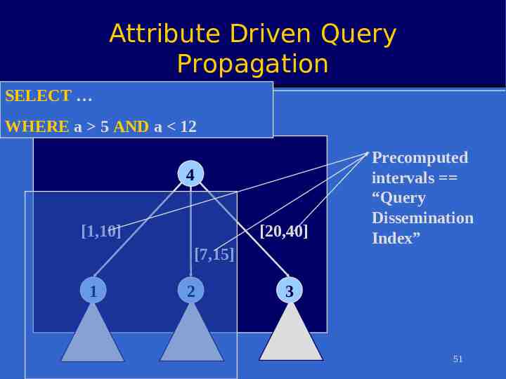
Attribute Driven Query Propagation SELECT WHERE a 5 AND a 12 4 [1,10] [20,40] [7,15] 1 2 Precomputed intervals “Query Dissemination Index” 3 51

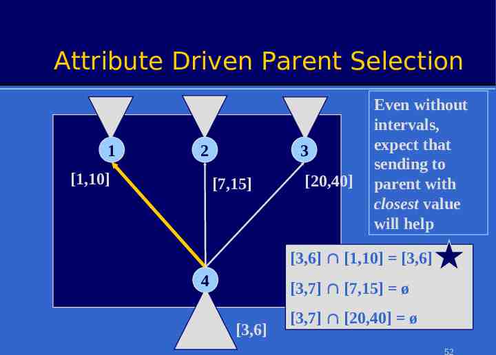
Attribute Driven Parent Selection 1 2 [1,10] 3 [7,15] [20,40] Even without intervals, expect that sending to parent with closest value will help [3,6] [1,10] [3,6] 4 [3,7] [7,15] ø [3,6] [3,7] [20,40] ø 52

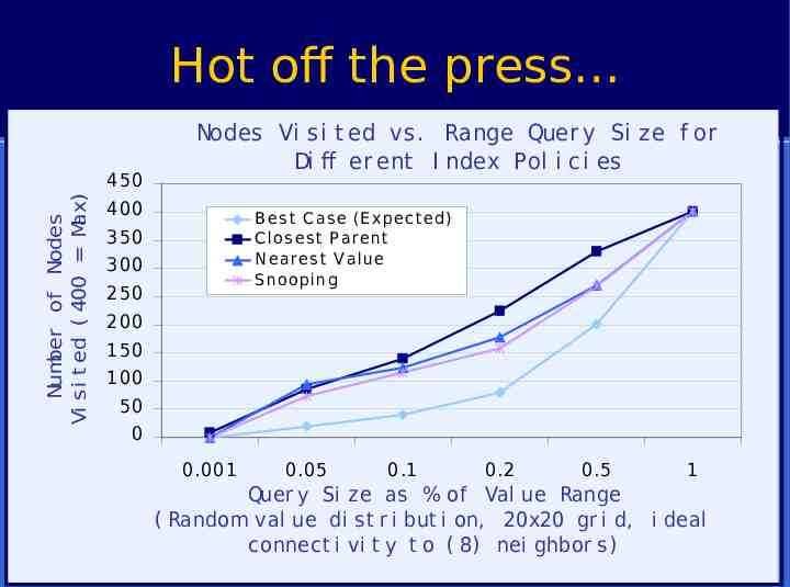
Hot off the press Number of Nodes Vi si t ed ( 400 Max) 450 Nodes Vi s i t ed vs . Range Quer y Si z e f or Di ff er ent I ndex Pol i ci es 400 B es t C as e (E x pec ted) C los es t P arent N eares t V alue S nooping 350 300 250 200 150 100 50 0 0.001 0.05 0.1 0.2 0.5 1 Quer y Si z e as % of Val ue Range ( Random val ue di s t r i but i on, 20x20 gr i d, i deal connect i vi t y t o ( 8) nei ghbor s ) 53

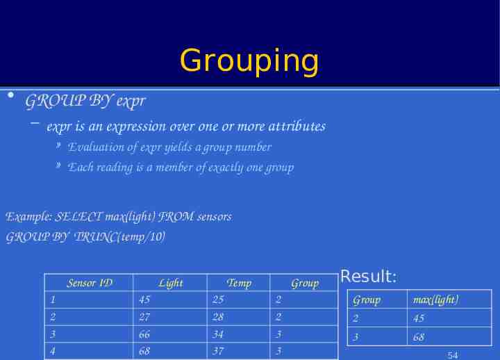
Grouping GROUP BY expr – expr is an expression over one or more attributes » Evaluation of expr yields a group number » Each reading is a member of exactly one group Example: SELECT max(light) FROM sensors GROUP BY TRUNC(temp/10) Sensor ID 1 2 3 4 Light 45 27 66 68 Temp 25 28 34 37 Group 2 2 3 3 Result: Group 2 3 max(light) 45 68 54

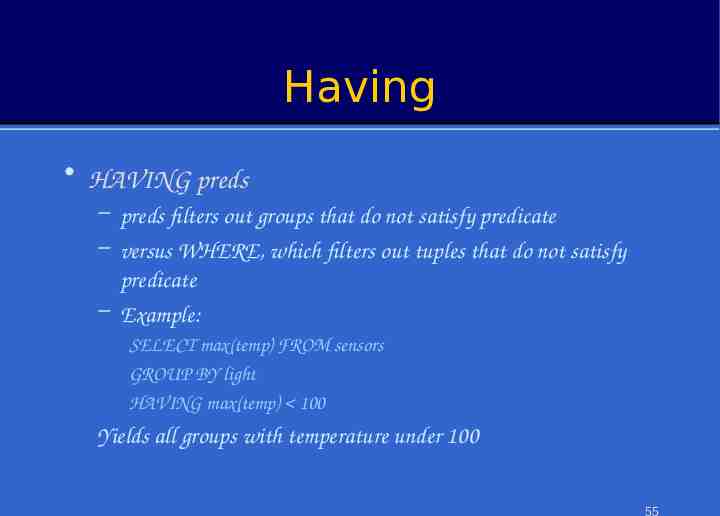
Having HAVING preds – preds filters out groups that do not satisfy predicate – versus WHERE, which filters out tuples that do not satisfy predicate – Example: SELECT max(temp) FROM sensors GROUP BY light HAVING max(temp) 100 Yields all groups with temperature under 100 55

Group Eviction Problem: Number of groups in any one iteration may exceed available storage on sensor Solution: Evict! – Choose one or more groups to forward up tree – Rely on nodes further up tree, or root, to recombine groups properly – What policy to choose? » Intuitively: least popular group, since don’t want to evict a group that will receive more values this epoch. » Experiments suggest: Policy matters very little Evicting as many groups as will fit into a single message is good 56

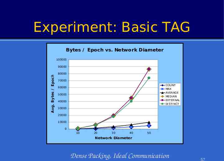
Experiment: Basic TAG Bytes / Epoch vs. Network Diameter 100000 Avg. Bytes / Epoch 90000 80000 70000 COUNT MAX AVERAGE MEDIAN EXTERNAL DISTINCT 60000 50000 40000 30000 20000 10000 0 10 20 30 40 50 Network Diameter Dense Packing, Ideal Communication 57

Experiment: Hypothesis Testing Messages/ Epoch vs. Network Diameter 3000 Messages / Epoch 2500 2000 No Guess Guess 50 Guess 90 Snooping 1500 1000 500 0 10 20 30 40 50 Network Diameter Uniform Value Distribution, Dense Packing, Ideal Communication 58

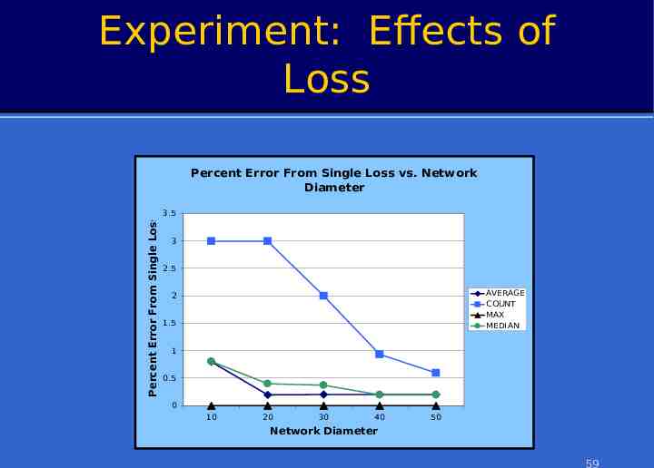
Experiment: Effects of Loss Percent Error From Single Loss Percent Error From Single Loss vs. Network Diameter 3.5 3 2.5 AVERAGE COUNT MAX MEDI AN 2 1.5 1 0.5 0 10 20 30 40 50 Network Diameter 59

Experiment: Benefit of Cache Percentage of Network I nvolved vs. Network Diameter 1.2 % Netw ork 1 0.8 No Cache 5 Rounds Cache 9 Rounds Cache 15 Rounds Cache 0.6 0.4 0.2 0 10 20 30 40 50 Network Diameter 60

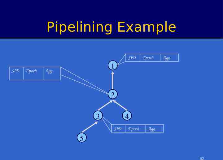
Pipelined Aggregates After query propagates, during each epoch: – Each sensor samples local sensors once Value from 2 produced at – Combines them with PSRs from children – Outputs PSR representing aggregate state in the previous time t arrives at 1 at time epoch. (t 1) 2 After (d-1) epochs, PSR for the whole tree output at root – d Depth of the routing tree – If desired, partial state from top k levels could be output in kth epoch To avoid combining PSRs from different epochs, sensors must cache values from children 1 3 4 5 Value from 5 produced at time t arrives at 1 at time (t 3)61

Pipelining Example SID SID Epoch Epoch Agg. 1 Agg. 2 3 4 SID Epoch Agg. 5 62

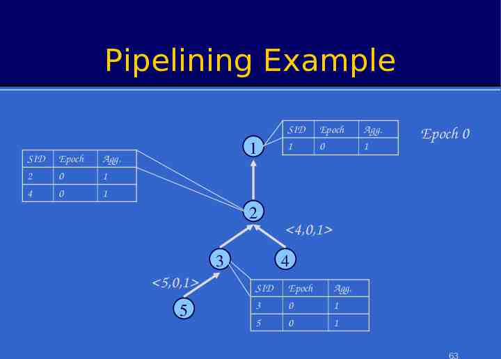
Pipelining Example SID Epoch Agg. 2 0 1 4 0 1 1 2 3 5,0,1 5 SID Epoch Agg. 1 0 1 Epoch 0 4,0,1 4 SID Epoch Agg. 3 0 1 5 0 1 63

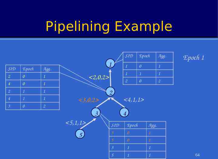
Pipelining Example SID Epoch Agg. 2 0 1 4 0 1 2 1 1 4 1 1 3 0 2 1 2,0,2 3,0,2 2 3 5,1,1 5 SID Epoch Agg. 1 0 1 1 1 1 2 0 2 Epoch 1 4,1,1 4 SID Epoch Agg. 3 0 1 5 0 1 3 1 1 5 1 1 64

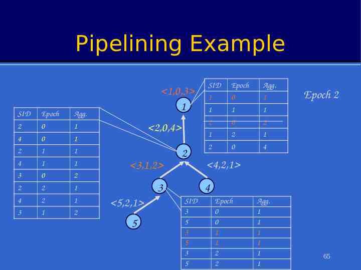
Pipelining Example SID Epoch Agg. 2 0 1 4 0 1 2 1 1 4 1 1 3 0 2 2 2 1 4 2 1 3 1 2 1,0,3 1 2,0,4 3,1,2 2 3 5,2,1 5 SID Epoch Agg. 1 0 1 1 1 1 2 0 2 1 2 1 2 0 4 Epoch 2 4,2,1 4 SID 3 5 3 5 3 5 Epoch 0 0 1 1 2 2 Agg. 1 1 1 1 1 1 65

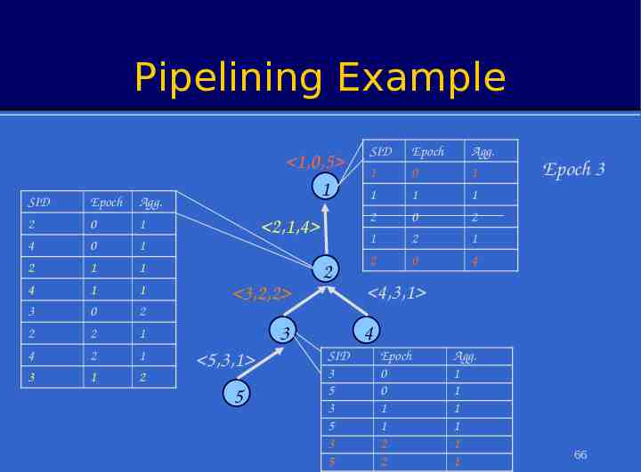
Pipelining Example SID Epoch Agg. 2 0 1 4 0 1 2 1 1 4 1 1 3 0 2 2 2 1 4 2 1 3 1 2 1,0,5 1 2,1,4 3,2,2 2 3 5,3,1 5 SID Epoch Agg. 1 0 1 1 1 1 2 0 2 1 2 1 2 0 4 Epoch 3 4,3,1 4 SID 3 5 3 5 3 5 Epoch 0 0 1 1 2 2 Agg. 1 1 1 1 1 1 66

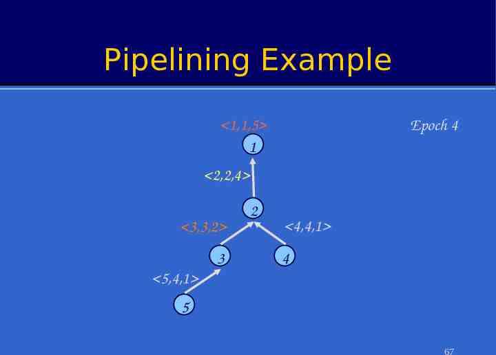
Pipelining Example Epoch 4 1,1,5 1 2,2,4 3,3,2 3 2 4,4,1 4 5,4,1 5 67

Our Stream Semantics One stream, ‘sensors’ We control data rates Joins between that stream and buffers are allowed Joins are always landmark, forward in time, one tuple at a time – Result of queries over ‘sensors’ either a single tuple (at time of query) or a stream Easy to interface to more sophisticated systems Temporal aggregates enable fancy window operations 68

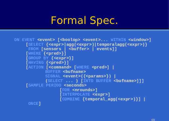
Formal Spec. ON EVENT event [ boolop event . WITHIN window ] [SELECT { expr agg( expr ) temporalagg( expr )} FROM [sensors buffer events]] [WHERE { pred }] [GROUP BY { expr }] [HAVING { pred }] [ACTION [ command [WHERE pred ] BUFFER bufname SIGNAL event ({ params }) (SELECT . ) [INTO BUFFER bufname ]]] [SAMPLE PERIOD seconds [FOR nrounds ] [INTERPOLATE expr ] [COMBINE {temporal agg( expr )}] ONCE] 69

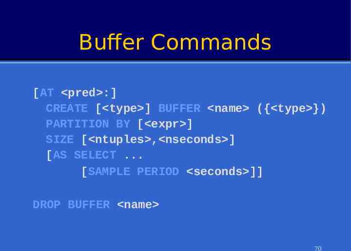
Buffer Commands [AT pred :] CREATE [ type ] BUFFER name ({ type }) PARTITION BY [ expr ] SIZE [ ntuples , nseconds ] [AS SELECT . [SAMPLE PERIOD seconds ]] DROP BUFFER name 70