SPSS Workshop Day 2 – Data Analysis

SPSS Workshop Day 2 – Data Analysis

Outline Descriptive Statistics Types of data Graphical Summaries – For Categorical Variables – For Quantitative Variables Contingency Tables Hypothesis Testing – One Sample t-test – Two Sample t-test Sample Size/Power Analysis

Descriptive Statistics 5-number summary – – – – – Minimum- minimum value in your dataset Q1- 25th percentile (25% of the data is below this value) Median- middle value of your data (50th percentile: 50% of the data is below this value) Q3- 75th percentile (75% of the data is below this value) Maximum- maximum value in your dataset Mean- average value of your all your data points Standard deviation- the average distance each observation falls from the mean Variance- average of the squared deviations; explains the variation of the data about the mean

To SPSS: Open gssnet.sav - Analyze- Descriptive Statistics - Descriptives - Analyze- Descriptive Statistics- Frequencies (you can get more descriptive statistics here also)

Types of Data Variable- any characteristic that is recorded for subjects in a study – Categorical- if each observation belongs to one of a set of categories – Quantitative- if observations on it take numerical values that represent different magnitudes of the variable Discrete- if its possible values form a set of separate numbers, such as 0, 1, 2, Continuous- if its possible values form an interval

Other Valuable Terminology Parameter- a numerical summary of the population Statistic- a numerical summary of a sample taken from the population Frequency table- a listing of possible values for a variable, together with the number of observations for each value – Relative frequency- proportions and percentages

Graphical Summaries for Categorical Variables Pie chart- a circle having a “slice of the pie” for each category. The size of a slice corresponds to the percentage of observations in the category Bar chart- displays a vertical bar for each category. The height of the bar is the percentage of observations in the category

To SPSS: Still in gssnet.sav For the pie chart: - Graphs- Pie- Summaries of groups of cases- Define slices by netcat- Click OK For labels: - Double click on the chart - Elements- Show data labels- choose labels

SPSS continued For the bar chart: - Graphs- Bar- Simple - Category axis: netcat Again, we can choose which labels to appear on the chart by double clicking.

Graphical Summaries for Quantitative Variables Dot plot- shows a dot for each observation, placed just above the value on the number line for that observation. Stem-and-Leaf Plot- each observation is represented by a stem and a leaf. Usually the stem consists of all digits except the final one, which is the leaf. Histogram- a graph that uses bars to portray the frequencies or the relative frequencies of the possible outcomes. Scatterplot- display for two variables. It uses the horizontal axis for the explanatory variable (x) and the vertical axis for the response variable (y).

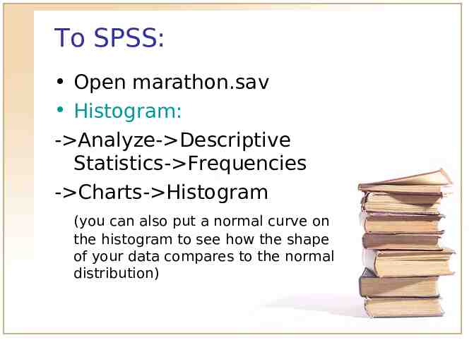
To SPSS: Open marathon.sav Histogram: - Analyze- Descriptive Statistics- Frequencies - Charts- Histogram (you can also put a normal curve on the histogram to see how the shape of your data compares to the normal distribution)

SPSS continued: Scatterplots: - Graphs- Scatter/dot. - Simple Scatter- Define - Choose (continuous) variables

Other Useful Plots Time plot- charts each observation, on the vertical scale, against the time it was measured, on the horizontal scale Box plot- constructed from the 5-number summary

To SPSS: Box plots: - Graphs- Boxplot- Simple - variable (continuous) - category axis (categorical) (You can also use boxplots in order to visually compare different groups on a quantitative variable, i.e. age by gender)

Contingency Tables/Cross Tabs A contingency table is a display for two categorical variables. Its rows list the categories of one variable and its columns list the categories of the other variable. Each entry in the table is the frequency of cases in the sample with certain outcomes of the two variables The process of taking a data file and finding the frequencies for the cells of a contingency table is referred to as crosstabulation of the data

Example 2 x 2 contingency table: Binge Drinking by Gender Binge Drinker Nonbinge Drinker Total Male 1908 2017 3925 Female 2854 4125 6979 Total 4762 6142 10904

Chi-squared Test for Independence The chi-squared test is a hypothesis test to see whether two categorical variables are independent of one another. H 0 : variables are independent H 1 : variables are not independent We will look to see if the p-value .05 (Reject the null hypothesis) If so, then our variables are not independent of one another

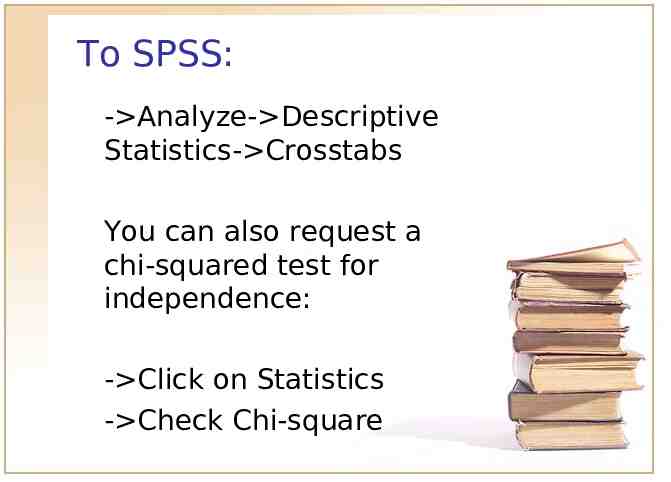
To SPSS: - Analyze- Descriptive Statistics- Crosstabs You can also request a chi-squared test for independence: - Click on Statistics - Check Chi-square

Interpreting P-values We compare the calculated p-value to a pre-specified value (usually .05), if the calculated p-value is less than .05 then there is significant evidence to reject the null hypothesis.

One-sample t-test Does the population mean differ from hypothesized value? – Different alternative hypotheses H1: 0 H1: 0 H 1 : 0 (SPSS only does two-sided hypothesis test)

Examples Does anorexia therapy induce a positive mean weight change ? H1: 0 Is the amount of Coke dispensed H 1 :into 12a can 12 oz.? Do radio advertisements increase the average daily sales of hamburgers? H 1 : 1500

To SPSS: Is the mean age of marathon runners greater than 30? - Analyze- Compare means - One sample ttest - test value 30

Interpreting the p-value With a p-value less than .05, there is a significant difference between the mean age of our sample and the specified test value of 30.

Two-sample t-test (Independent samples) Does one population mean differ from another population mean? – Different alternative hypotheses H1 : 1 2 1 2 0 H1 : 1 2 1 2 0 H1 : 1 2 1 2 0

Examples Do women tend to spend more time on housework than men? H1 : 1 2 1 2 0 Do men and women watch the same amount of television in a day? H1 : 1 2 1 2 0

To SPSS: Are the male runners older than the female runners? - Analyze- Independent Samples t-test - test variable (continuous) - grouping variable (categorical)

Interpreting the p-value With a p-value less than .05, there is a significant difference between the mean completion time for males and females.

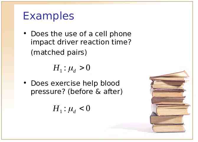
Paired t-test (matched pairs/dependent samples) Does the population mean change for two different treatments (before & after)? – Different alternative hypotheses H1 : d 0 H1 : d 0 H1 : d 0

Examples Does the use of a cell phone impact driver reaction time? (matched pairs) H1 : d 0 Does exercise help blood pressure? (before & after) H1 : d 0

To SPSS: Open endorph.sav Do the beta endorphin levels differ before and after running a halfmarathon? - Analyze- Compare means - Paired samples t-test - Paired variables (before & after)

Interpreting the p-value With a p-value less than .05, there is a significant difference between beta endorphin levels before and after running a half-marathon.

Determining Sample Size Power- the ability to reject the null hypothesis when it is false – If a certain level of power is desired, use power analysis to determine the required sample size