Sparrow Light Scattering (LS) Analysis Tool The first flight ver.

Sparrow Light Scattering (LS) Analysis Tool The first flight ver. 1.04 March 26, 2010

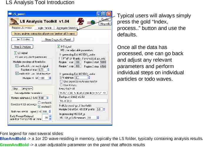
LS Analysis Tool Introduction The main analysis is done in the Process LS Events tab and consists of 3 steps: (1) Index (2) Process (3) Categorize

LS Analysis Tool Introduction Typical users will always simply press the gold “Index, process.” button and use the defaults. Once all the data has processed, one can go back and adjust any relevant parameters and perform individual steps on individual particles or todo waves. Font legend for next several slides: BlueAndBold - a 1or 2D wave residing in memory, typically the LS folder, typically containing analysis results. GreenAndBold - a user-adjustable parameter on the panel that affects results

Step 1. Index At the step the user is prompted for the folder containing the DAQ LS data files. These files are named yymmdd xxxxxxxxx lsSt.hdf. Diagnostic values are loaded into waves and global variables are set based on the DAQ settings. Users can view and modify the global variables in the Diagnostic Panel. So far the code only allows for analysis of LS data taken with the same DAQ settings (i.e min and max range of m/z sticks, PToF calibration values, etc.). Along with global variables, the index step also creates some waves: msChop PTOF 1e-6*(DataDelay PulserPeriod*CoAdds*p), for plotting spectra data vs time msChop mz amus mzStartVal p, for plotting spectra data vs m/z.

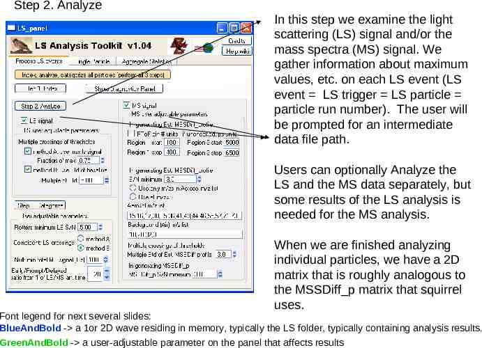
Step 2. Analyze In this step we examine the light scattering (LS) signal and/or the mass spectra (MS) signal. We gather information about maximum values, etc. on each LS event (LS event LS trigger LS particle particle run number). The user will be prompted for an intermediate data file path. Users can optionally Analyze the LS and the MS data separately, but some results of the LS analysis is needed for the MS analysis. When we are finished analyzing individual particles, we have a 2D matrix that is roughly analogous to the MSSDiff p matrix that squirrel uses. Font legend for next several slides: BlueAndBold - a 1or 2D wave residing in memory, typically the LS folder, typically containing analysis results. GreenAndBold - a user-adjustable parameter on the panel that affects results

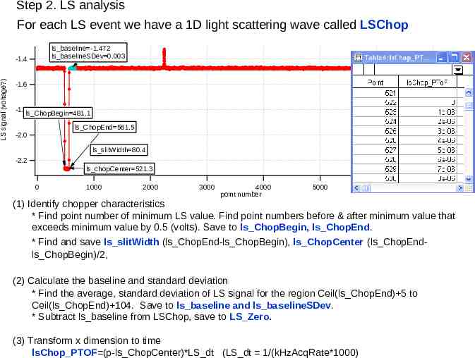
Step 2. LS analysis For each LS event we have a 1D light scattering wave called LSChop LS signal (voltage?) -1.4 -1.6 -1.8 -2.0 -2.2 0 1000 2000 3000 4000 point number 5000 6000 7000 The main analysis tasks for each LS signal are: (1) Identify chopper characteristics (start, center, end) (2) Calculate a baseline and the standard deviation of a non-signal region. (3) Translate the x-dimension from point number to time. (4) Find the maximum LS signal and associated statistics. (5) Estimate the number of particles seen in this single LS event (nominally1).

Step 2. LS analysis For each LS event we have a 1D light scattering wave called LSChop ls baseline -1.472 ls baselineSDev 0.003 LS signal (voltage?) -1.4 -1.6 -1.8ls ChopBegin 481.1 ls ChopEnd 561.5 -2.0 ls slitWidth 80.4 -2.2 ls chopCenter 521.3 0 1000 2000 3000 4000 point number 5000 6000 7000 (1) Identify chopper characteristics * Find point number of minimum LS value. Find point numbers before & after minimum value that exceeds minimum value by 0.5 (volts). Save to ls ChopBegin, ls ChopEnd. * Find and save ls slitWidth (ls ChopEnd-ls ChopBegin), ls ChopCenter (ls ChopEndls ChopBegin)/2, (2) Calculate the baseline and standard deviation * Find the average, standard deviation of LS signal for the region Ceil(ls ChopEnd) 5 to Ceil(ls ChopEnd) 104. Save to ls baseline and ls baselineSDev. * Subtract ls baseline from LSChop, save to LS Zero. (3) Transform x dimension to time lsChop PTOF (p-ls ChopCenter)*LS dt (LS dt 1/(kHzAcqRate*1000)

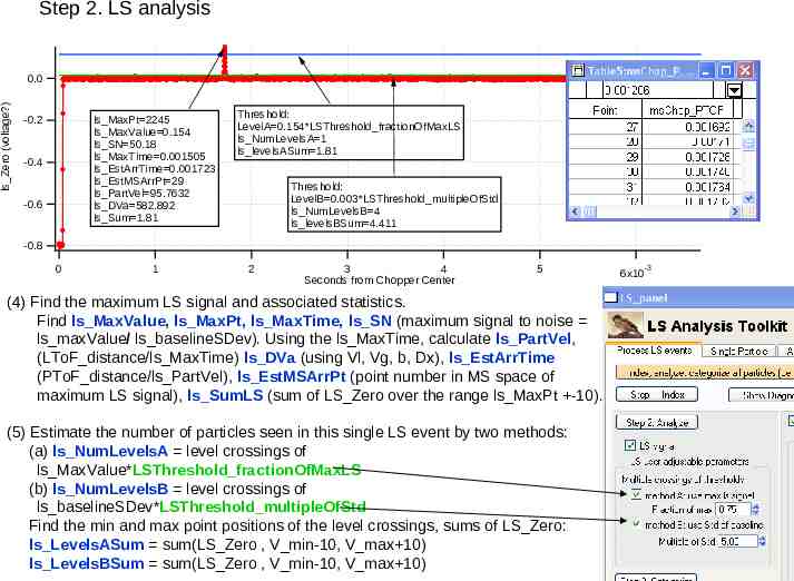
Step 2. LS analysis ls Zero (voltage?) 0.0 ls MaxPt 2245 ls MaxValue 0.154 ls SN 50.18 ls MaxTime 0.001505 ls EstArrTime 0.001723 ls EstMSArrPt 29 ls PartVel 95.7632 ls DVa 582.892 ls Sum 1.81 -0.2 -0.4 -0.6 Threshold: LevelA 0.154*LSThreshold fractionOfMaxLS ls NumLevelsA 1 ls levelsASum 1.81 Threshold: LevelB 0.003*LSThreshold multipleOfStd ls NumLevelsB 4 ls levelsBSum 4.411 -0.8 0 1 2 3 4 Seconds from Chopper Center 5 (4) Find the maximum LS signal and associated statistics. Find ls MaxValue, ls MaxPt, ls MaxTime, ls SN (maximum signal to noise ls maxValue/ ls baselineSDev). Using the ls MaxTime, calculate ls PartVel, (LToF distance/ls MaxTime) ls DVa (using Vl, Vg, b, Dx), ls EstArrTime (PToF distance/ls PartVel), ls EstMSArrPt (point number in MS space of maximum LS signal), ls SumLS (sum of LS Zero over the range ls MaxPt -10). (5) Estimate the number of particles seen in this single LS event by two methods: (a) ls NumLevelsA level crossings of ls MaxValue*LSThreshold fractionOfMaxLS (b) ls NumLevelsB level crossings of ls baselineSDev*LSThreshold multipleOfStd Find the min and max point positions of the level crossings, sums of LS Zero: ls LevelsASum sum(LS Zero , V min-10, V max 10) ls LevelsBSum sum(LS Zero , V min-10, V max 10) 6x10 -3

Step 2, MS analysis For each LS event we have a 2D mass spectra stick matrix called sp Stick. 280 280 260 m/z 46 profile m/z 47 profile 240 240 220 200 PToF Bin number PToF Bin Number 200 160 120 One column - PToF m/z profile 180 160 140 120 100 80 80 60 40 40 20 0 0 800 10 20 30 40 50 60 70 80 90 1000 1200 ms signal m/z One row - PToF bin spectra PToF Bin #117 PToF Bin #110 MS signal 1200 1000 800 600 400 200 10 20 30 40 50 60 m/z 70 80 90 100 The main analysis tasks for the 2D MS sp stick matrix are: (1) Apply a DC-marker type of correction to get the signal with the zero removed (2) Identify the PToF time in which the MS sees a particle (3) Generate a single mass spectra

Step 2. MS analysis (1) Apply a DC-marker type of correction to get the MS signal with the background removed. * Apply duty cycle correction to sp Stick (*sqrt(28/mz)). It is not necessary to perform this correction at the very beginning; we simply do it first to get it out of the way. * For each m/z extract the PToF m/z profile. Find the average and standard deviation of the first 25 bins beginning with MSPToFBinOffset; put result in ms mz Vavg1, ms mz Vsdev. Find the average of the last 25 bins, put result in ms mz Vavg2. Subtract the average of ms mz Vavg1, ms mz Vavg1 from the mz Profile; call this entity ms zero profile. Put ms mz zero profile in ptof stick p for this m/z (for later possible squirrel use). 280 240 ms mz vAvg2 563.1 200 m/z 46 profile ms mz avg 160 120 80 ms mz vAvg1 559.9 msChop mz Vsdev 8.3 40 240 PToF Bin number PToF Bin number 280 200m/z 46 ms zero profile 160 120 80 40 0 0 600 800 1000 ms signal 0 500 ms signal (DC marker corrected)

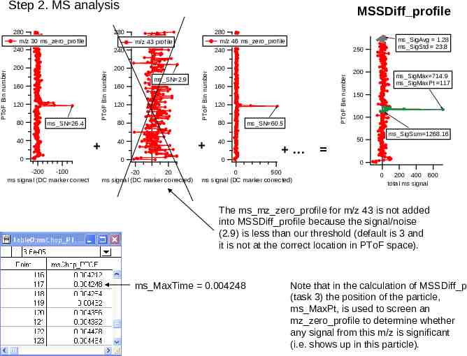
Step 2. MS analysis (2) Identify the PToF time in which the MS sees a particle. To accomplish this task, we generate a 1-D wave called MSSDiff profile. MSSDiff profile is the 2D matrix sp Stick that has been collapsed in m/z dimension. See next slide for graphics. For each ms mz zero profile find the maximum value after MSPToFBinOffset, ms mz Vmax, the bin number of the maximum value, ms mz VmaxLoc, and the signal to noise ms mz SN (ms mz Vmax/ms mzVsdev). If ms mz SN MSThreshold multipleOfStd (a) if considering only m/zs in mzAerosolList add to MSSDiff profile (b) else don’t screen for mz aerosols, just add to MSSDiff profile. * Using MSSDiff profile (a sum of baseline subtracted profiles of various mzs) Find the average and standard deviation for the last 25 PToF bins; put results in ms SigAvg, ms SigStd. * Find the max value, ms SigMax, the maximum PToF bin number ms MaxPt , and the signal to noise, ms SigMaxOverStd (ms sigMax/ms sigStd). * Find the time of the maximum MS signal via ms SigMaxPt and msChop PTOF, ms SigMaxTime. * Using the ms SigMaxTime and the PToF distance, find the particle velocity ms PartVel. * Estimate overall signal at max value, ms SigSum, (sum of MSSDiff profile over the range ms MaxPt -5). * Estimate the number of particles seen in this single LS event by level crossings of MSSDiff profile by ms SigStd*MSThreshold multipleOfStd

MSSDiff profile 280 240 280 m/z 46 ms zero profile 240 200 200 200 160 120 80 40 0 ms SN 26.4 ms SN 2.9 160 120 80 PToF Bin number m/z 43 profile 40 0 160 120 80 40 ms SN 60.5 0 -200 -100 -20 20 ms signal (DC marker corrected) ms signal (DC marker corrected) ms SigAvg 1.28 ms SigStd 23.8 250 PToF Bin number 280 m/z 30 ms zero profile 240 PToF Bin number PToF Bin number Step 2. MS analysis 200 ms SigMax 714.9 ms SigMaxPt 117 150 100 ms SigSum 1268.16 50 0 0 500 ms signal (DC marker corrected) 0 200 400 600 total ms signal The ms mz zero profile for m/z 43 is not added into MSSDiff profile because the signal/noise (2.9) is less than our threshold (default is 3 and it is not at the correct location in PToF space). ms MaxTime 0.004248 Note that in the calculation of MSSDiff p (task 3) the position of the particle, ms MaxPt, is used to screen an mz zero profile to determine whether any signal from this m/z is significant (i.e. shows up in this particle).

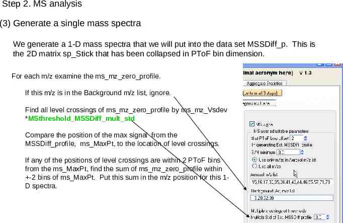
Step 2. MS analysis (3) Generate a single mass spectra We generate a 1-D mass spectra that we will put into the data set MSSDiff p. This is the 2D matrix sp Stick that has been collapsed in PToF bin dimension. For each m/z examine the ms mz zero profile. If this m/z is in the Background m/z list, ignore. Find all level crossings of ms mz zero profile by ms mz Vsdev *MSthreshold MSSDiff mult std Compare the position of the max signal from the MSSDiff profile, ms MaxPt, to the location of level crossings. If any of the positions of level crossings are within 2 PToF bins from the ms MaxPt, find the sum of ms mz zero profile within -2 bins of ms MaxPt. Put this sum in the m/z position for this 1D spectra.

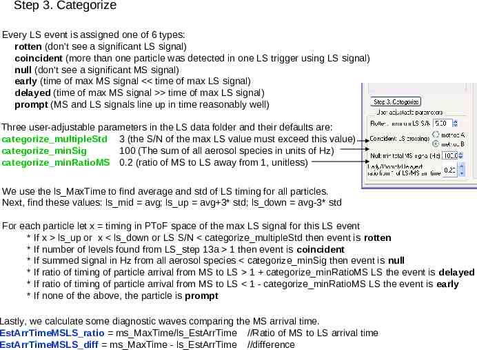
Step 3. Categorize Every LS event is assigned one of 6 types: rotten (don’t see a significant LS signal) coincident (more than one particle was detected in one LS trigger using LS signal) null (don’t see a significant MS signal) early (time of max MS signal time of max LS signal) delayed (time of max MS signal time of max LS signal) prompt (MS and LS signals line up in time reasonably well) Three user-adjustable parameters in the LS data folder and their defaults are: categorize multipleStd 3 (the S/N of the max LS value must exceed this value) categorize minSig 100 (The sum of all aerosol species in units of Hz) categorize minRatioMS 0.2 (ratio of MS to LS away from 1, unitless) We use the ls MaxTime to find average and std of LS timing for all particles. Next, find these values: ls mid avg; ls up avg 3* std; ls down avg-3* std For each particle let x timing in PToF space of the max LS signal for this LS event * If x ls up or x ls down or LS S/N categorize multipleStd then event is rotten * If number of levels found from LS step 13a 1 then event is coincident * If summed signal in Hz from all aerosol species categorize minSig then event is null * If ratio of timing of particle arrival from MS to LS 1 categorize minRatioMS LS the event is delayed * If ratio of timing of particle arrival from MS to LS 1 - categorize minRatioMS LS the event is early * If none of the above, the particle is prompt Lastly, we calculate some diagnostic waves comparing the MS arrival time. EstArrTimeMSLS ratio ms MaxTime/ls EstArrTime //Ratio of MS to LS arrival time EstArrTimeMSLS diff ms MaxTime - ls EstArrTime //difference

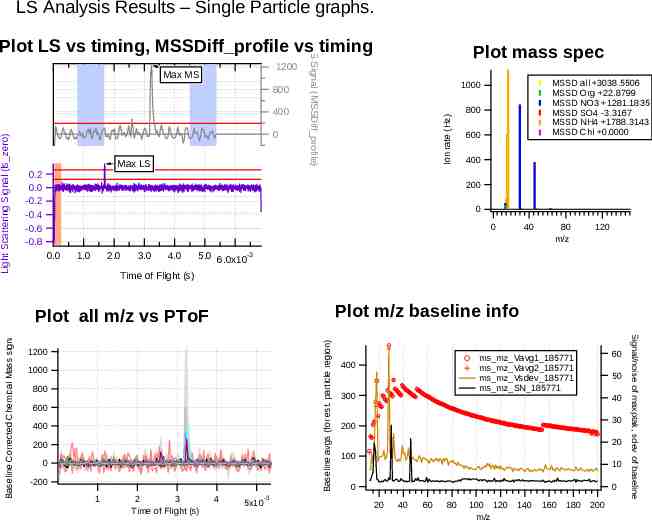
LS Analysis Results The results of the analysis can be viewed on a single particle or in aggregate. The utility of viewing the analysis results of a single particle is to verify calculations, examine useradjustable values, etc. Particles are identified by their number (simply the row entry) or by the ‘particle run’ value. Many results are simply viewed as variable displays on the panel.

LS Analysis Results – Single Particle graphs. Plot LS vs timing, MSSDiff profile vs timing Light Scattering Signal (ls zero) 400 0 Max LS 0.2 0.0 -0.2 -0.4 -0.6 -0.8 800 600 400 200 0 0 0.0 1.0 2.0 3.0 4.0 40 80 m/z 120 5.0 6.0x10-3 Time of Flight (s) Plot m/z baseline info 1200 1000 800 600 400 200 0 -200 1 2 3 Time of Flight (s) 4 -3 5x10 60 ms mz Vavg1 185771 ms mz Vavg2 185771 ms mz Vsdev 185771 ms mz SN 185771 400 300 50 40 30 200 20 100 10 0 0 20 40 60 80 100 120 m/z 140 160 180 200 Signal/noise of maxptak, sdev of baseline Baseline avgs (for est. particle region) Plot all m/z vs PToF Baseline Corrected Chemical Mass signal MSSD all 3038.5506 MSSD Org 22.8799 MSSD NO3 1281.1835 MSSD SO4 -3.3167 MSSD NH4 1788.3143 MSSD Chl 0.0000 1000 Ion rate (Hz) 800 MS Signal (MSSDiff profile) 1200 Max MS Plot mass spec

Prompt Delayed Early -3 3.5x10 Null RottenLS Coincident Prompt 3.0 2.5 2.0 2.0 2.5 3.0 3.5 4.0 4.5x10-3 Chopper-MS(s), Time of max signal Hist prompt Hist delayed Hist early Hist null Hist coincident 100 frequency Chopper-LS(s), Est Arrival Time to MS LS Analysis Results – Aggregate Statistics. 80 60 40 20 0 200 300 400 LS Dva (nm) 500 600

Some caveats about LS Tool version 1.3 Some of the important squirrel panel tools work. Currently there is not a capability to perform and LS analysis when important DAQ settings such as the number of m/z per spectra or the number of PToF bins have changed between DAQ hdf files. Currently there is not a capability to convert to ug/m3. This isn’t conceptually difficult, but because we don’t record the flow, etc. at every LS event, squirrel will need to be adjusted to ‘find’ these values. The code hasn’t been tested on large data sets ( 10,000 particles). For users of the earlier version of the code, v 1.2, many waves have been renamed and many waves moved to intermediate files to try to conserve memory. One may use many tools in the MS tab, particularly the time series and average mass spectra on any todo wave. One may generate PToF size distributions, PToF image plots, and PToF average mass spectra plots on the all todo wave. Performing some of these operations on some non-all todo waves may not work because once again squirrel expects some values to be present for all particles, and the DAQ only saves some values once per file (parVal vl, vg, dx, b, etc). The x-axis for image plots currently corresponds to particle number (instead of time). This will eventually change. The Aggregate Statistics section is quite minimal, but will grow as the standard experience of the community evolves. User suggestions and contributions are VERY welcome! Most of the current tools have to do with generating basic statistics about the data and insuring that the instrument was working properly.