SIMULATION AND MONTE CARLO Some General Principles James C. Spall

SIMULATION AND MONTE CARLO Some General Principles James C. Spall Johns Hopkins University Applied Physics Laboratory August 2011

Overview Basic principles Advantages/disadvantages Classification of simulation models Role of sponsor and management in simulation study Verification, validation, and accreditation Pseudo random numbers and danger of replacing random variables by their means Parallel and distributed computing Example of Monte Carlo in computing integral What course will/will not cover Homework exercises Selected references 2

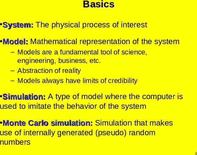
Basics System: The physical process of interest Model: Mathematical representation of the system – Models are a fundamental tool of science, engineering, business, etc. – Abstraction of reality – Models always have limits of credibility Simulation: A type of model where the computer is used to imitate the behavior of the system Monte Carlo simulation: Simulation that makes use of internally generated (pseudo) random numbers 3

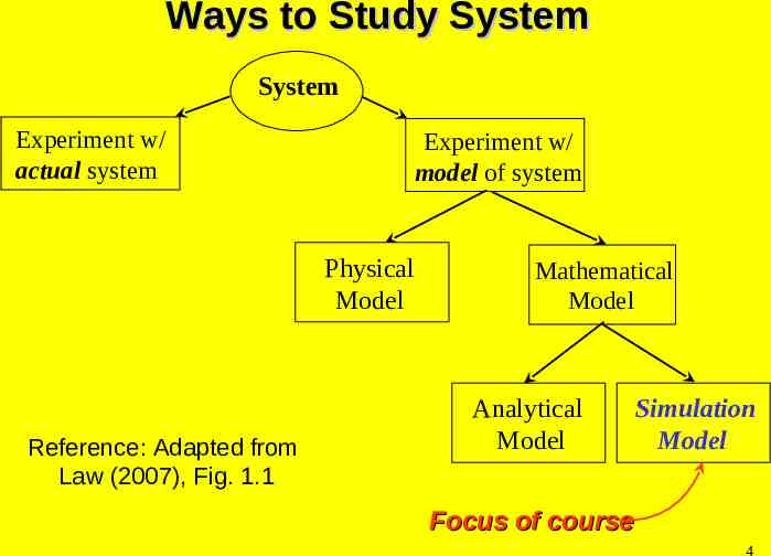
Ways to Study System System Experiment w/ actual system Experiment w/ model of system Physical Model Reference: Adapted from Law (2007), Fig. 1.1 Mathematical Model Analytical Model Simulation Model Focus of course 4

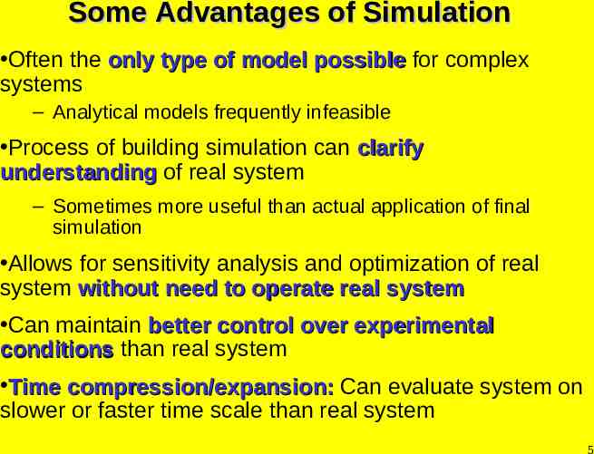
Some Advantages of Simulation Often the only type of model possible for complex systems – Analytical models frequently infeasible Process of building simulation can clarify understanding of real system – Sometimes more useful than actual application of final simulation Allows for sensitivity analysis and optimization of real system without need to operate real system Can maintain better control over experimental conditions than real system Time compression/expansion: Can evaluate system on slower or faster time scale than real system 5

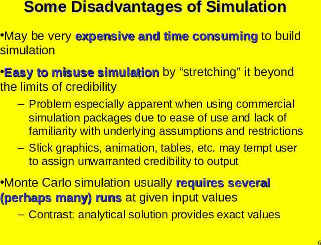
Some Disadvantages of Simulation May be very expensive and time consuming to build simulation Easy to misuse simulation by “stretching” it beyond the limits of credibility – Problem especially apparent when using commercial simulation packages due to ease of use and lack of familiarity with underlying assumptions and restrictions – Slick graphics, animation, tables, etc. may tempt user to assign unwarranted credibility to output Monte Carlo simulation usually requires several (perhaps many) runs at given input values – Contrast: analytical solution provides exact values 6

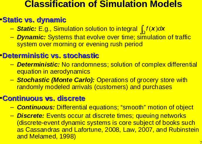
Classification of Simulation Models Static vs. dynamic – Static: E.g., Simulation solution to integral f ( x )dx – Dynamic: Systems that evolve over time; simulation of traffic system over morning or evening rush period Deterministic vs. stochastic – Deterministic: No randomness; solution of complex differential equation in aerodynamics – Stochastic (Monte Carlo): Operations of grocery store with randomly modeled arrivals (customers) and purchases Continuous vs. discrete – Continuous: Differential equations; “smooth” motion of object – Discrete: Events occur at discrete times; queuing networks (discrete-event dynamic systems is core subject of books such as Cassandras and Lafortune, 2008, Law, 2007, and Rubinstein and Melamed, 1998) 7

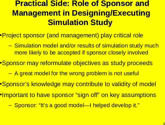
Practical Side: Role of Sponsor and Management in Designing/Executing Simulation Study Project sponsor (and management) play critical role – Simulation model and/or results of simulation study much more likely to be accepted if sponsor closely involved Sponsor may reformulate objectives as study proceeds – A great model for the wrong problem is not useful Sponsor’s knowledge may contribute to validity of model Important to have sponsor “sign off” on key assumptions – Sponsor: “It’s a good model—I helped develop it.” 8

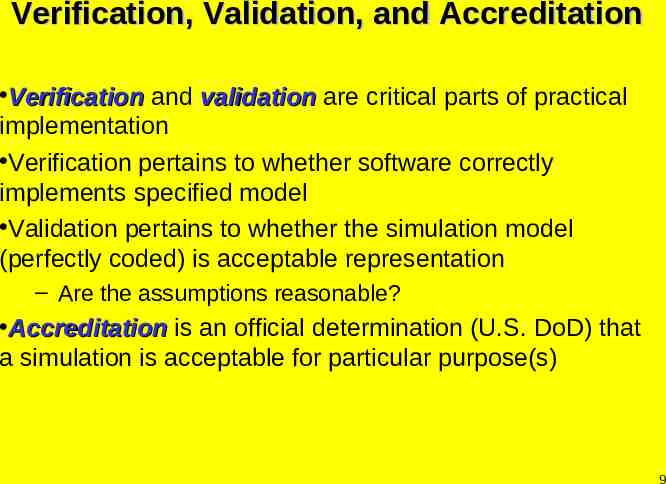
Verification, Validation, and Accreditation Verification and validation are critical parts of practical implementation Verification pertains to whether software correctly implements specified model Validation pertains to whether the simulation model (perfectly coded) is acceptable representation – Are the assumptions reasonable? Accreditation is an official determination (U.S. DoD) that a simulation is acceptable for particular purpose(s) 9

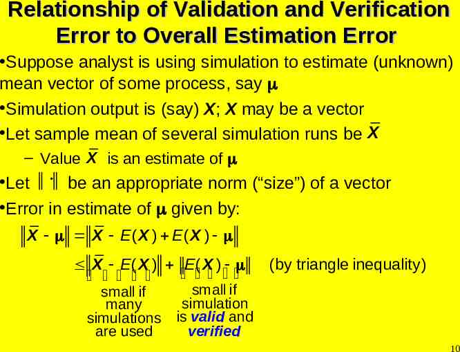
Relationship of Validation and Verification Error to Overall Estimation Error Suppose analyst is using simulation to estimate (unknown) mean vector of some process, say Simulation output is (say) X; X may be a vector Let sample mean of several simulation runs be X – Value X is an estimate of Let be an appropriate norm (“size”) of a vector Error in estimate of given by: X X E( X ) E( X ) X E( X ) E( X ) small if many simulations are used (by triangle inequality) small if simulation is valid and verified 10

Pseudo Random Number Generators Monte Carlo simulations usually based on computer generation of pseudo random numbers Starting point is generation of sequence of independent, identically distributed uniform (U(0, 1)) random variables – U(0, 1) random numbers of direct interest in some applications – More commonly, U(0, 1) numbers transformed to random numbers having other distributions (e.g., Poisson distribution for arrivals in a network) Computer-based random pseudo number generators produce deterministic and periodic sequence of numbers – Discussed in Appendix D and Chapter 16 of Spall (2003) Want pseudo random numbers that “look” random – Able to pass all relevant statistical tests for randomness 11

Danger of Replacing Random Variables by Their Means Suppose Monte Carlo simulation involves random process X Common simplification is to replace X by its mean – – – – Makes simulation easier to implement and interpret Can work with constants instead of probability distributions No need to specify forms of distributions No need to generate random outcomes X (may be difficult for non-standard distributions; see, e.g, Appendix D and Chap. 16 of Spall, 2003) – Easier output analysis as removes source of randomness However, simplification can lead to seriously incorrect results Example: Queuing system with random arrival/service times – Replacing randomness with mean arrival rate and service times may lead to very different (wrong) estimates of average wait time and/or number of customers in queue 12

Parallel and Distributed Simulation Simulation may be of little practical value if each run requires days or weeks – Practical simulations may easily require processing of 10 9 to 1012 events, each event requiring many computations Parallel and distributed (PAD) computation based on: Execution of large simulation on multiple processors connected through a network PAD simulation is large activity for researchers and practitioners in parallel computation (e.g., Chap. 12 by Fujimoto in Banks, 1998; Law, 2007, pp. 61–66) Distributed interactive simulation is closely related area; very popular in defense applications 13

Parallel and Distributed Simulation (cont’d) Parallel computation sometimes allows for much faster execution Two general roles for parallelization: – Split supporting roles (random number generation, event coordination, statistical analysis, etc.) – Decompose model into submodels (e.g., overall network into individual queues) Need to be able to decouple computing tasks Synchronization important—cause must precede effect! – Decoupling of airports in interconnected air traffic network difficult; may be inappropriate for parallel processing – Certain transaction processing systems (e.g., supermarket checkout, toll booths) easier for parallel processing 14

Parallel and Distributed Simulation (cont’d) Hardware platforms for implementation vary – Shared vs. distributed memory (all processors can directly access key variables vs. information is exchanged indirectly via “messages”) – Local area network (LAN) or wide area network (WAN) – Speed of light is limitation to rapid processing in WAN Distributed interactive simulation (DIS) is one common implementation of PAD simulation DIS very popular in defense applications – Geographically disbursed analysts can interact as in combat situations (LAN or WAN is standard platform) – Sufficiently important that training courses exist for DIS alone (e.g., www.simulation.com/Training) 15

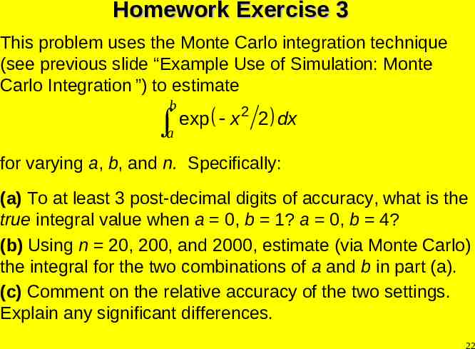
Example Use of Simulation: Monte Carlo Integration Common problem is estimation of f ( x )dx where f is a function, x is vector and is domain of integration – Monte Carlo integration popular for complex f and/or Special case: Estimate integration a, b One approach: b a f ( x )dx for scalar x, and limits of – Let p(u) denote uniform density function over [a, b] – Let Ui denote i th uniform random variable generated by Monte Carlo according to the density p(u) – Then, for “large” n: b a n a f ( x )dx n f (Ui ) i 1 b 16

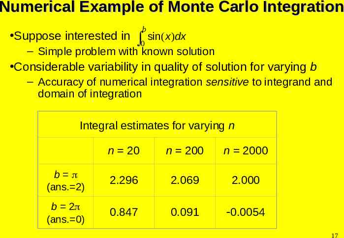
Numerical Example of Monte Carlo Integration Suppose interested in b 0 sin( x )dx – Simple problem with known solution Considerable variability in quality of solution for varying b – Accuracy of numerical integration sensitive to integrand and domain of integration Integral estimates for varying n n 20 n 200 n 2000 b (ans. 2) 2.296 2.069 2.000 b 2 (ans. 0) 0.847 0.091 0.0054 17

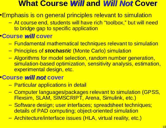
What Course Will and Will Not Cover Emphasis is on general principles relevant to simulation – At course end, students will have rich “toolbox,” but will need to bridge gap to specific application Course will cover – Fundamental mathematical techniques relevant to simulation – Principles of stochastic (Monte Carlo) simulation – Algorithms for model selection, random number generation, simulation-based optimization, sensitivity analysis, estimation, experimental design, etc. Course will not cover – Particular applications in detail – Computer languages/packages relevant to simulation (GPSS, Flexsim, SLAM, SIMSCRIPT, Arena, Simulink, etc.) – Software design; user interfaces; spreadsheet techniques; details of PAD computing; object-oriented simulation – Architecture/interface issues (HLA, virtual reality, etc.) 18

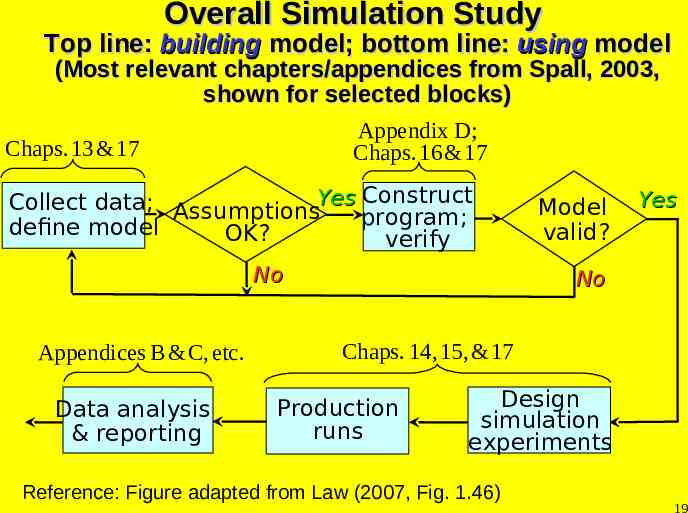
Overall Simulation Study Top line: building model; bottom line: using model (Most relevant chapters/appendices from Spall, 2003, shown for selected blocks) Appendix D; Chaps. 13 & 17 Chaps. 16 & 17 Collect data; AssumptionsYes Construct program; define model OK? verify No Appendices B & C, etc. Data analysis & reporting Model valid? Yes No Chaps. 14, 15, & 17 Production runs Design simulation experiments Reference: Figure adapted from Law (2007, Fig. 1.46) 19

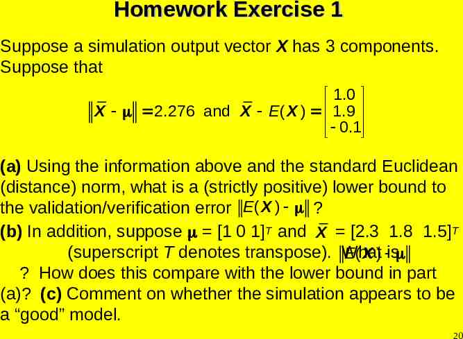
Homework Exercise 1 Suppose a simulation output vector X has 3 components. Suppose that 1.0 X 2.276 and X E ( X ) 1.9 0.1 (a) Using the information above and the standard Euclidean (distance) norm, what is a (strictly positive) lower bound to the validation/verification error E ( X ) ? (b) In addition, suppose [1 0 1]T and X [2.3 1.8 1.5]T (superscript T denotes transpose). What E ( X ) is ? How does this compare with the lower bound in part (a)? (c) Comment on whether the simulation appears to be a “good” model. 20

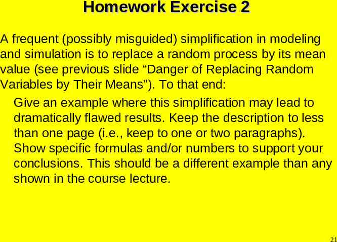
Homework Exercise 2 A frequent (possibly misguided) simplification in modeling and simulation is to replace a random process by its mean value (see previous slide “Danger of Replacing Random Variables by Their Means”). To that end: Give an example where this simplification may lead to dramatically flawed results. Keep the description to less than one page (i.e., keep to one or two paragraphs). Show specific formulas and/or numbers to support your conclusions. This should be a different example than any shown in the course lecture. 21

Homework Exercise 3 This problem uses the Monte Carlo integration technique (see previous slide “Example Use of Simulation: Monte Carlo Integration ”) to estimate b a exp x 2 2 dx for varying a, b, and n. Specifically: (a) To at least 3 post-decimal digits of accuracy, what is the true integral value when a 0, b 1? a 0, b 4? (b) Using n 20, 200, and 2000, estimate (via Monte Carlo) the integral for the two combinations of a and b in part (a). (c) Comment on the relative accuracy of the two settings. Explain any significant differences. 22

Selected General References in Simulation and Monte Carlo Arsham, H. (1998), “Techniques for Monte Carlo Optimizing,” Monte Carlo Methods and Applications, vol. 4, pp. 181 229. Banks, J. (ed.) (1998), Handbook of Simulation: Principles, Methodology, Advances, Applications, and Practice, Wiley, New York. Cassandras, C. G. and Lafortune, S. (2008), Introduction to Discrete Event Systems (2nd ed.), Springer, New York. Fu, M. C. (2002), “Optimization for Simulation: Theory vs. Practice” (with discussion by S. Andradóttir, P. Glynn, and J. P. Kelly), INFORMS Journal on Computing, vol. 14, pp. 192 227. Fu, M. C. and Hu, J.-Q. (1997), Conditional Monte Carlo: Gradient Estimation and Optimization Applications, Kluwer, Boston. Gosavi, A. (2003), Simulation-Based Optimization: Parametric Optimization Techniques and Reinforcement Learning, Kluwer, Boston. Law, A. M. (2007), Simulation Modeling and Analysis (4th ed.), McGraw-Hill, New York. Liu, J. S. (2001), Monte Carlo Strategies in Scientific Computing, Springer-Verlag, New York. Robert, C. P. and Casella, G. (2004), Monte Carlo Statistical Methods (2nd ed.), SpringerVerlag, New York. Rubinstein, R. Y. and Melamed, B. (1998), Modern Simulation and Modeling, Wiley, New York. Rubinstein, R. Y. and Kroese, D. P. (2007), Simulation and the Monte Carlo Method (2nd ed.), Wiley, New York. Spall, J. C. (2003), Introduction to Stochastic Search and Optimization, Wiley, Hoboken, NJ. 23