Reinforcement Learning Andrew W. Moore Associate Professor School

Reinforcement Learning Andrew W. Moore Associate Professor School of Computer Science Carnegie Mellon University Note to other teachers and users of these slides. Andrew would be delighted if you found this source material useful in giving your own lectures. Feel free to use these slides verbatim, or to modify them to fit your own needs. PowerPoint originals are available. If you make use of a significant portion of these slides in your own lecture, please include this message, or the following link to the source repository of Andrew’s tutorials: http://www.cs.cmu.edu/ awm/tutori als . Comments and corrections gratefully received. www.cs.cmu.edu/ awm [email protected] 412-268-7599 Copyright 2002, Andrew W. Moore April 23rd, 2002

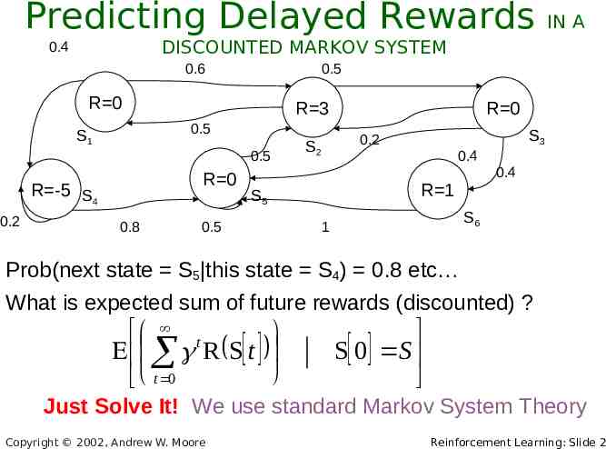
Predicting Delayed Rewards DISCOUNTED MARKOV SYSTEM 0.4 0.6 0.5 R 0 R 3 0.5 S1 0.5 R 0 R -5 S4 0.2 IN A 0.8 S3 0.2 S2 0.4 0.4 R 1 S5 0.5 R 0 S6 1 Prob(next state S5 this state S4) 0.8 etc What is expected sum of future rewards (discounted) ? t R S t t 0 S 0 S Just Solve It! We use standard Markov System Theory Copyright 2002, Andrew W. Moore Reinforcement Learning: Slide 2

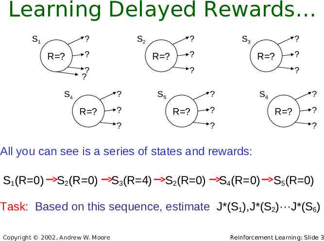
Learning Delayed Rewards S1 ? R ? S2 ? ? R ? ? ? S4 ? ? R ? ? ? R ? S3 ? S5 ? ? R ? ? ? S6 ? ? R ? ? ? ? All you can see is a series of states and rewards: S1(R 0) S2(R 0) S3(R 4) S2(R 0) S4(R 0) S5(R 0) Task: Based on this sequence, estimate J*(S1),J*(S2)···J*(S6) Copyright 2002, Andrew W. Moore Reinforcement Learning: Slide 3

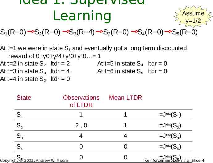
Idea 1: Supervised Learning S1(R 0) S2(R 0) S3(R 4) S2(R 0) Assume γ 1/2 S4(R 0) S5(R 0) At t 1 we were in state S1 and eventually got a long term discounted reward of 0 γ0 γ24 γ30 γ40 1 At t 2 in state S2 ltdr 2 At t 5 in state S4 ltdr 0 At t 3 in state S3 ltdr 4 At t 6 in state S5 ltdr 0 At t 4 in state S2 ltdr 0 State Observations of LTDR Mean LTDR S1 1 1 Jest(S1) S2 2,0 1 Jest(S2) S3 4 4 Jest(S3) S4 0 0 Jest(S4) 0 0 S5 2002, Andrew W. Moore Copyright est J (S5) Reinforcement Learning: Slide 4

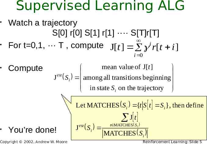
Supervised Learning ALG Watch a trajectory S[0] r[0] S[1] r[1] ···· S[T]r[T] For t 0,1, ··· T , compute J[t ] i r[t i ] i 0 Compute mean value of J[t ] est J Si among all transitions beginning in state S on the trajectory i Let MATCHES S i {t S t S i }, then define You’re done! Copyright 2002, Andrew W. Moore J est Si J t t MATCHES S i MATCHES S i Reinforcement Learning: Slide 5

Supervised Learning ALG for the timid If you have an anxious personality you may be worried about edge effects for some of the final transitions. With large trajectories these are negligible. Copyright 2002, Andrew W. Moore Reinforcement Learning: Slide 6

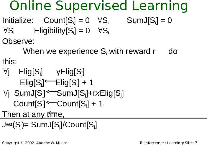
Online Supervised Learning Initialize: Count[Si] 0 Si SumJ[Si] 0 Si Eligibility[Si] 0 Si Observe: When we experience Si with reward r do this: j Elig[Sj] γElig[Sj] Elig[Sj] Elig[Sj] 1 j SumJ[Sj] SumJ[Sj] rxElig[Sj] Count[Si] Count[Si] 1 Then at any time, Jest(Sj) SumJ[Sj]/Count[Sj] Copyright 2002, Andrew W. Moore Reinforcement Learning: Slide 7

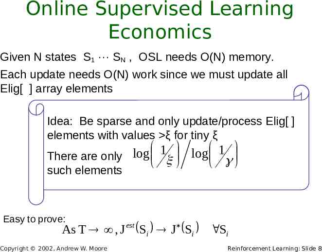
Online Supervised Learning Economics Given N states S1 ··· SN , OSL needs O(N) memory. Each update needs O(N) work since we must update all Elig[ ] array elements Idea: Be sparse and only update/process Elig[ ] elements with values ξ for tiny ξ 1 log 1 log There are only such elements Easy to prove: As T , J est Si J Si Si Copyright 2002, Andrew W. Moore Reinforcement Learning: Slide 8

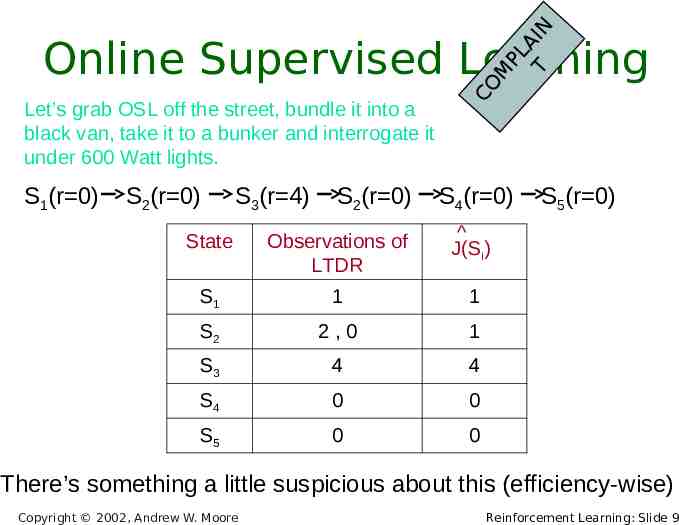
PL A T IN Let’s grab OSL off the street, bundle it into a black van, take it to a bunker and interrogate it under 600 Watt lights. S1(r 0) S2(r 0) S3(r 4) S2(r 0) CO M Online Supervised Learning S4(r 0) State Observations of LTDR J(Si) S1 1 1 S2 2,0 1 S3 4 4 S4 0 0 S5 0 0 S5(r 0) There’s something a little suspicious about this (efficiency-wise) Copyright 2002, Andrew W. Moore Reinforcement Learning: Slide 9

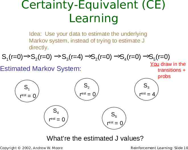
Certainty-Equivalent (CE) Learning Idea: Use your data to estimate the underlying Markov system, instead of trying to estimate J directly. S1(r 0) S2(r 0) S3(r 4) S2(r 0) S4(r 0) S5(r 0) You draw in the transitions probs Estimated Markov System: S1 rest 0 S4 r est 0 S2 S3 rest 0 rest 4 S5 rest 0 What’re the estimated J values? Copyright 2002, Andrew W. Moore Reinforcement Learning: Slide 10

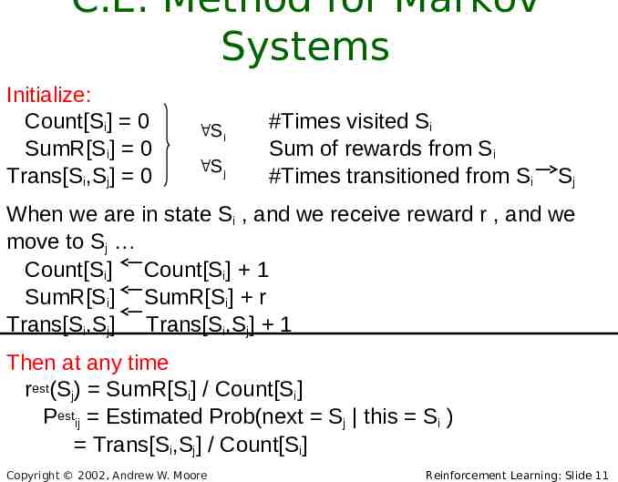
C.E. Method for Markov Systems Initialize: Count[Si] 0 SumR[Si] 0 Trans[Si,Sj] 0 Si Sj #Times visited Si Sum of rewards from Si #Times transitioned from Si Sj When we are in state Si , and we receive reward r , and we move to Sj Count[Si] Count[Si] 1 SumR[Si] SumR[Si] r Trans[Si,Sj] Trans[Si,Sj] 1 Then at any time rest(Sj) SumR[Si] / Count[Si] Pestij Estimated Prob(next Sj this Si ) Trans[Si,Sj] / Count[Si] Copyright 2002, Andrew W. Moore Reinforcement Learning: Slide 11

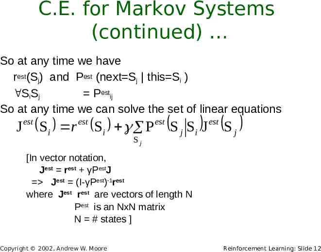
C.E. for Markov Systems (continued) So at any time we have rest(Sj) and Pest (next Sj this Si ) SiSj Pestij So at any time we can solve the set of linear equations J est Si r Si P S j Si J S j est est est Sj [In vector notation, Jest rest γPestJ Jest (I-γPest)-1rest where Jest rest are vectors of length N Pest is an NxN matrix N # states ] Copyright 2002, Andrew W. Moore Reinforcement Learning: Slide 12

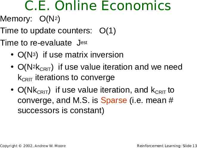
C.E. Online Economics Memory: O(N2) Time to update counters: O(1) Time to re-evaluate Jest O(N3) if use matrix inversion O(N2kCRIT) if use value iteration and we need kCRIT iterations to converge O(NkCRIT) if use value iteration, and kCRIT to converge, and M.S. is Sparse (i.e. mean # successors is constant) Copyright 2002, Andrew W. Moore Reinforcement Learning: Slide 13

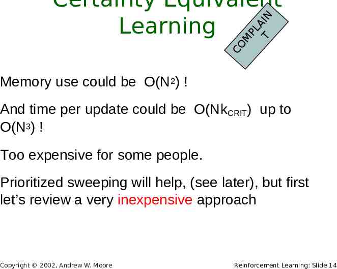
CO M PL A T IN Certainty Equivalent Learning Memory use could be O(N2) ! And time per update could be O(NkCRIT) up to O(N3) ! Too expensive for some people. Prioritized sweeping will help, (see later), but first let’s review a very inexpensive approach Copyright 2002, Andrew W. Moore Reinforcement Learning: Slide 14

Why this obsession with onlineiness? I really care about supplying up-to-date Jest estimates all the time. Can you guess why? If not, all will be revealed in good time Copyright 2002, Andrew W. Moore Reinforcement Learning: Slide 15

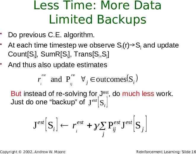
Less Time: More Data Limited Backups Do previous C.E. algorithm. At each time timestep we observe Si(r) Sj and update Count[Si], SumR[Si], Trans[Si,Sj] And thus also update estimates ri est est and Pij j outcomes Si But instead of re-solving for Jest, do much less work. Just do one “backup” of J est Si J est Si riest Pijest J est S j j Copyright 2002, Andrew W. Moore Reinforcement Learning: Slide 16

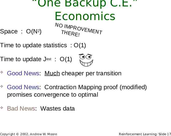
“One Backup C.E.” Economics Space : O(N2) NO IMP ROVEM ENT THERE ! Time to update statistics : O(1) Time to update Jest : O(1) Good News: Much cheaper per transition Good News: Contraction Mapping proof (modified) promises convergence to optimal Bad News: Wastes data Copyright 2002, Andrew W. Moore Reinforcement Learning: Slide 17

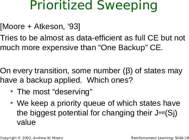
Prioritized Sweeping [Moore Atkeson, ’93] Tries to be almost as data-efficient as full CE but not much more expensive than “One Backup” CE. On every transition, some number (β) of states may have a backup applied. Which ones? The most “deserving” We keep a priority queue of which states have the biggest potential for changing their Jest(Sj) value Copyright 2002, Andrew W. Moore Reinforcement Learning: Slide 18

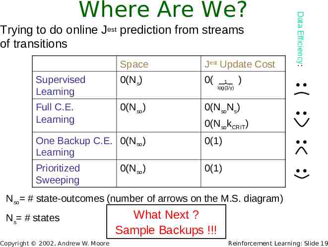
Trying to do online Jest prediction from streams of transitions Space Jest Update Cost Supervised Learning 0(Ns) 0( Full C.E. Learning 0(Nso) 0(NsoNs) 1 log(1/γ) ) 0(NsokCRIT) Data Efficiency: Where Are We? One Backup C.E. 0(Nso) Learning 0(1) Prioritized Sweeping 0(1) 0(Nso) Nso # state-outcomes (number of arrows on the M.S. diagram) Ns # states Copyright 2002, Andrew W. Moore What Next ? Sample Backups !!! Reinforcement Learning: Slide 19

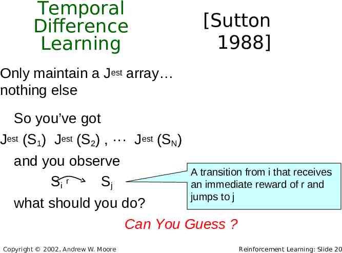
Temporal Difference Learning [Sutton 1988] Only maintain a Jest array nothing else So you’ve got Jest (S1) Jest (S2) , ··· Jest (SN) and you observe Si r Sj A transition from i that receives an immediate reward of r and jumps to j what should you do? Can You Guess ? Copyright 2002, Andrew W. Moore Reinforcement Learning: Slide 20

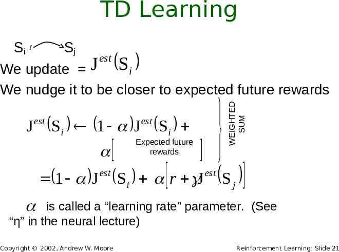
TD Learning Si r Sj est J est est WEIGHTED SUM We update J Si We nudge it to be closer to expected future rewards Si 1 J Si 1 J est Si r J est S j Expected future rewards is called a “learning rate” parameter. (See “η” in the neural lecture) Copyright 2002, Andrew W. Moore Reinforcement Learning: Slide 21

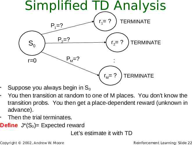
Simplified TD Analysis r1 ? P1 ? S0 P2 ? r 0 PM ? TERMINATE r2 ? TERMINATE : r M ? TERMINATE Suppose you always begin in S0 You then transition at random to one of M places. You don’t know the transition probs. You then get a place-dependent reward (unknown in advance). Then the trial terminates. Define J*(S0) Expected reward Let’s estimate it with TD Copyright 2002, Andrew W. Moore Reinforcement Learning: Slide 22

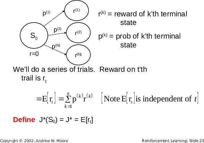
r(1) p(1) S0 p(2) r(2) · · · p(N) r 0 r(k) reward of k’th terminal state p(k) prob of k’th terminal state r(N) We’ll do a series of trials. Reward on t’th trail is rt n rt p k r k k 1 Note rt is independent of t Define J*(S0) J* E[rt] Copyright 2002, Andrew W. Moore Reinforcement Learning: Slide 23

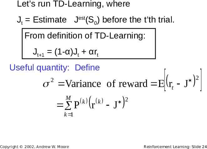
Let’s run TD-Learning, where Jt Estimate Jest(S0) before the t’th trial. From definition of TD-Learning: Jt 1 (1-α)Jt αrt Useful quantity: Define Variance of reward rt J 2 M P k 1 Copyright 2002, Andrew W. Moore k r k J 2 2 Reinforcement Learning: Slide 24

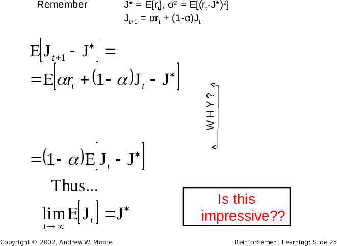
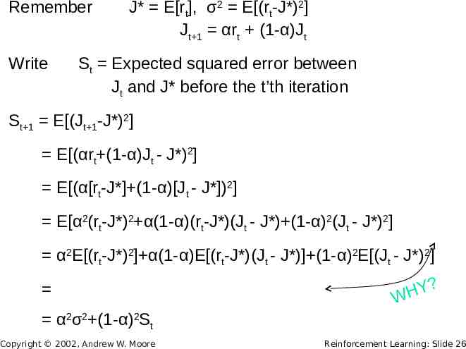
Remember J J* E[rt], σ2 E[(rt-J*)2] Jt 1 αrt (1-α)Jt t 1 J r 1 J t J WHY? t 1 J t J Thus. lim J t J t Copyright 2002, Andrew W. Moore Is this impressive? Reinforcement Learning: Slide 25

Remember Write J* E[rt], σ2 E[(rt-J*)2] Jt 1 αrt (1-α)Jt St Expected squared error between Jt and J* before the t’th iteration St 1 E[(Jt 1-J*)2] E[(αrt (1-α)Jt - J*)2] E[(α[rt-J*] (1-α)[Jt - J*])2] E[α2(rt-J*)2 α(1-α)(rt-J*)(Jt - J*) (1-α)2(Jt - J*)2] α2E[(rt-J*)2] α(1-α)E[(rt-J*)(Jt - J*)] (1-α)2E[(Jt - J*)2] Y? H W α2σ2 (1-α)2St Copyright 2002, Andrew W. Moore Reinforcement Learning: Slide 26

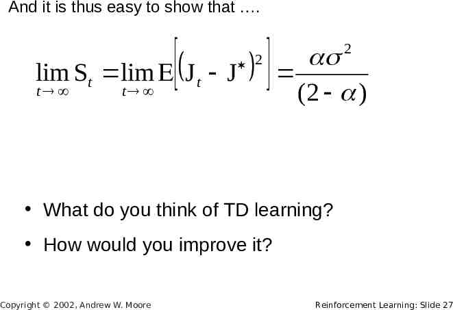
And it is thus easy to show that . lim St lim J t J t t 2 2 (2 ) What do you think of TD learning? How would you improve it? Copyright 2002, Andrew W. Moore Reinforcement Learning: Slide 27

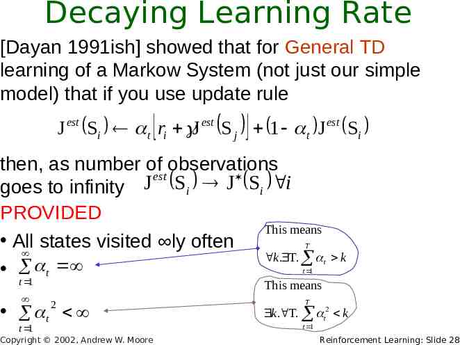
Decaying Learning Rate [Dayan 1991ish] showed that for General TD learning of a Markow System (not just our simple model) that if you use update rule J est Si t ri J est S j 1 t J est Si then, as number of observations est Si i J S J goes to infinity i PROVIDED This means All states visited ly often k . T. t T t k t 1 t 1 This means 2 t t 1 Copyright 2002, Andrew W. Moore T k . T. t2 k t 1 Reinforcement Learning: Slide 28

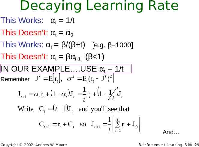
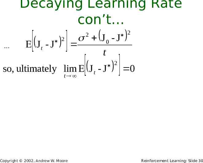
Decaying Learning Rate This Works: αt 1/t This Doesn’t: αt α0 This Works: αt β/(β t) [e.g. β 1000] This Doesn’t: αt βαt-1 (β 1) IN OUR EXAMPLE .USE αt 1/t Remember J rt , 2 (rt J ) 2 1 J t 1 t rt 1 t J t rt 1 1 J t t t Write Ct t 1 J t and you' ll see that 1 t Ct 1 rt Ct so J t 1 rt J 0 t i 1 Copyright 2002, Andrew W. Moore And Reinforcement Learning: Slide 29

Decaying Learning Rate con’t Jt - J 2 J 0 - J t 2 so, ultimately lim J t - J t Copyright 2002, Andrew W. Moore 2 0 2 Reinforcement Learning: Slide 30

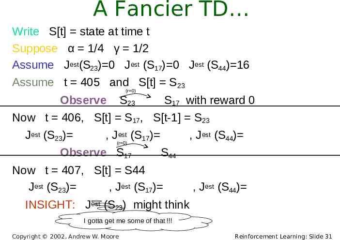
A Fancier TD Write S[t] state at time t Suppose α 1/4 γ 1/2 Assume Jest(S23) 0 Jest (S17) 0 Jest (S44) 16 Assume t 405 and S[t] S23 (r 0) Observe S23 S17 with reward 0 Now t 406, S[t] S17, S[t-1] S23 Jest (S23) est (S ) , J(r 0) 17 Observe S17 , Jest (S44) S44 Now t 407, S[t] S44 Jest (S23) , Jest (S17) , Jest (S44) INSIGHT: Jest (S23) might think I gotta get me some of that !!! Copyright 2002, Andrew W. Moore Reinforcement Learning: Slide 31

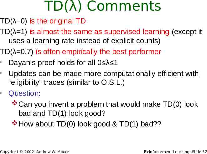
TD(λ) Comments TD(λ 0) is the original TD TD(λ 1) is almost the same as supervised learning (except it uses a learning rate instead of explicit counts) TD(λ 0.7) is often empirically the best performer Dayan’s proof holds for all 0 λ 1 Updates can be made more computationally efficient with “eligibility” traces (similar to O.S.L.) Question: Can you invent a problem that would make TD(0) look bad and TD(1) look good? How about TD(0) look good & TD(1) bad? Copyright 2002, Andrew W. Moore Reinforcement Learning: Slide 32

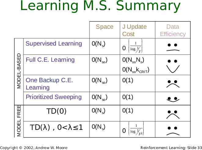
Learning M.S. Summary MODEL FREE MODEL-BASED Space Supervised Learning 0(Ns) Full C.E. Learning 0(Nso) J Update Cost 0 1 log 1 0(NsoNs) Data Efficiency 0(NsokCRIT) One Backup C.E. Learning 0(Nso) 0(1) Prioritized Sweeping 0(Nso) 0(1) TD(0) 0(Ns) 0(1) TD(λ) , 0 λ 1 0(Ns) Copyright 2002, Andrew W. Moore 0 1 log 1 Reinforcement Learning: Slide 33

Learning Policies for MDPs See previous lecture slides for definition of and computation with MDPs. The Heart of FORCEMENT REIN Learning state Copyright 2002, Andrew W. Moore Reinforcement Learning: Slide 34

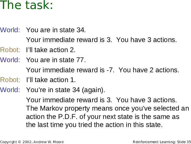
The task: World: You are in state 34. Your immediate reward is 3. You have 3 actions. Robot: I’ll take action 2. World: You are in state 77. Your immediate reward is -7. You have 2 actions. Robot: I’ll take action 1. World: You’re in state 34 (again). Your immediate reward is 3. You have 3 actions. The Markov property means once you’ve selected an action the P.D.F. of your next state is the same as the last time you tried the action in this state. Copyright 2002, Andrew W. Moore Reinforcement Learning: Slide 35

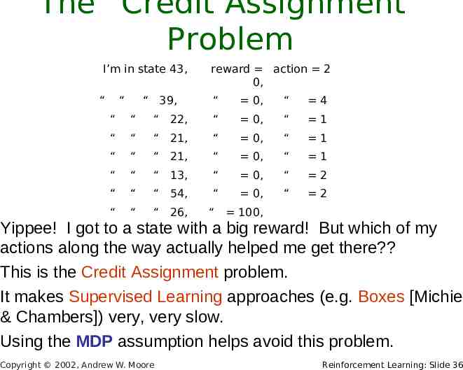
The “Credit Assignment” Problem I’m in state 43, “ “ “ 39, reward action 2 0, “ 0, “ 4 “ “ “ 22, “ 0, “ 1 “ “ “ 21, “ 0, “ 1 “ “ “ 21, “ 0, “ 1 “ “ “ 13, “ 0, “ 2 “ “ “ 54, “ 0, “ 2 “ “ “ 26, “ 100, Yippee! I got to a state with a big reward! But which of my actions along the way actually helped me get there? This is the Credit Assignment problem. It makes Supervised Learning approaches (e.g. Boxes [Michie & Chambers]) very, very slow. Using the MDP assumption helps avoid this problem. Copyright 2002, Andrew W. Moore Reinforcement Learning: Slide 36

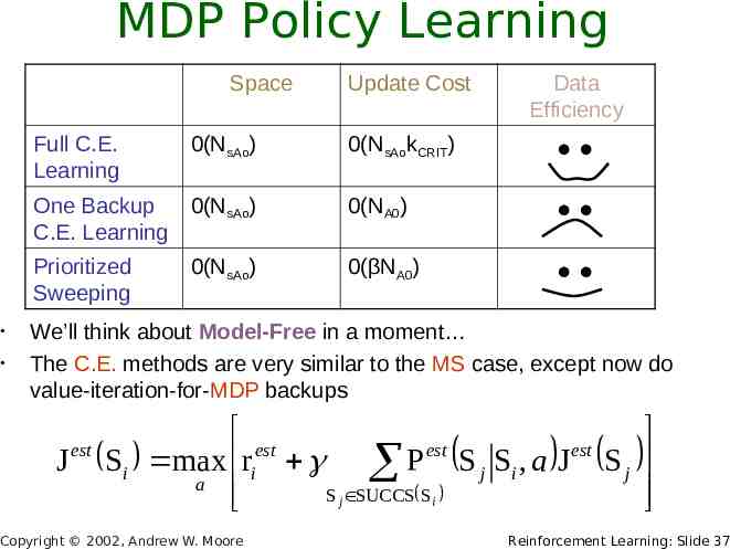
MDP Policy Learning Space Update Cost Data Efficiency Full C.E. Learning 0(NsAo) 0(NsAokCRIT) One Backup C.E. Learning 0(NsAo) 0(NΑ0) Prioritized Sweeping 0(NsAo) 0(βNΑ0) We’ll think about Model-Free in a moment The C.E. methods are very similar to the MS case, except now do value-iteration-for-MDP backups est est est J Si max ri P S j Si , a J S j a S j SUCCS Si est Copyright 2002, Andrew W. Moore Reinforcement Learning: Slide 37

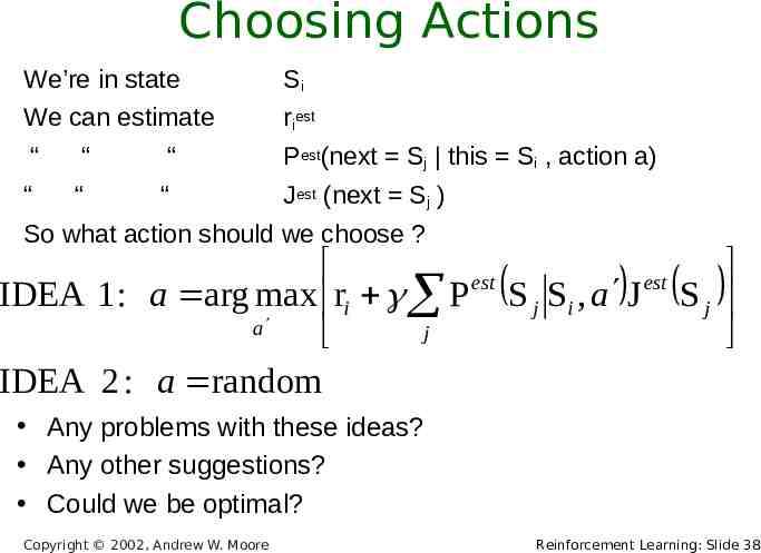
Choosing Actions We’re in state Si We can estimate riest “ “ “ Pest(next Sj this Si , action a) “ “ “ Jest (next Sj ) So what action should we choose ? est est IDEA 1 : a arg max ri P S j Si , a J S j a j IDEA 2 : a random Any problems with these ideas? Any other suggestions? Could we be optimal? Copyright 2002, Andrew W. Moore Reinforcement Learning: Slide 38

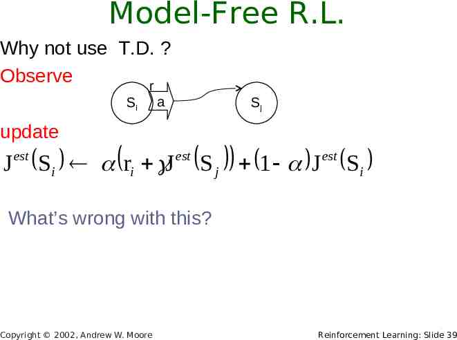
Model-Free R.L. Why not use T.D. ? Observe r Si a Sj update J est Si ri J est S j 1 J est Si What’s wrong with this? Copyright 2002, Andrew W. Moore Reinforcement Learning: Slide 39

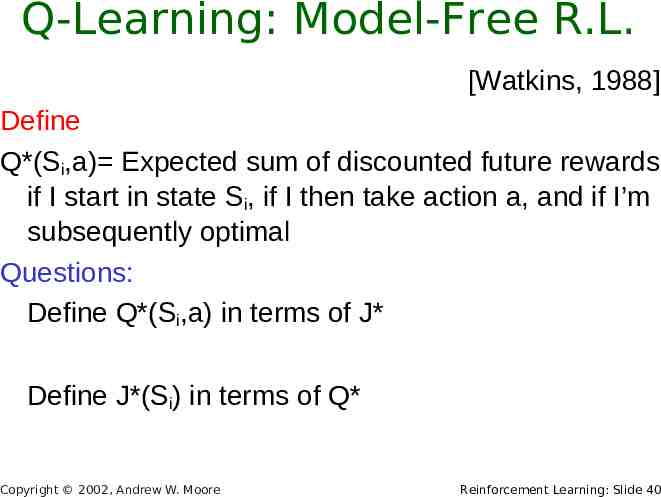
Q-Learning: Model-Free R.L. [Watkins, 1988] Define Q*(Si,a) Expected sum of discounted future rewards if I start in state Si, if I then take action a, and if I’m subsequently optimal Questions: Define Q*(Si,a) in terms of J* Define J*(Si) in terms of Q* Copyright 2002, Andrew W. Moore Reinforcement Learning: Slide 40

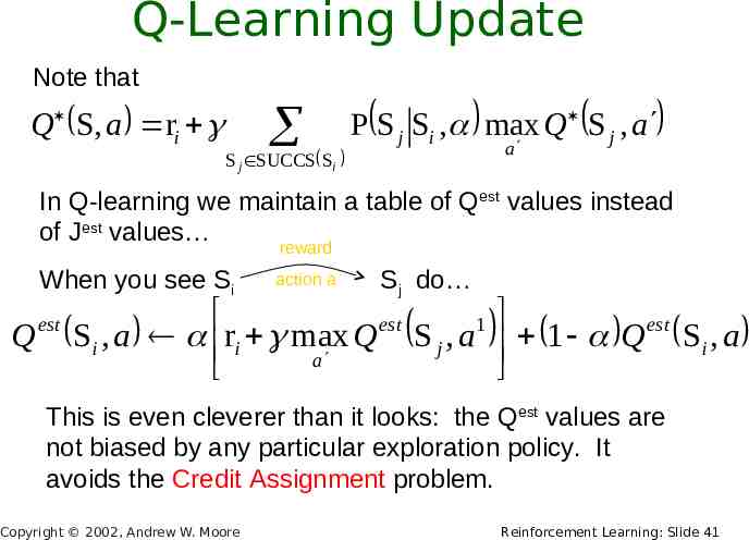
Q-Learning Update Note that Q S, a ri P S j Si , max Q S j , a a S j SUCCS Si In Q-learning we maintain a table of Qest values instead of Jest values reward When you see Si action a Sj do est 1 Q Si , a ri max Q S j , a 1 Q est Si , a a est This is even cleverer than it looks: the Qest values are not biased by any particular exploration policy. It avoids the Credit Assignment problem. Copyright 2002, Andrew W. Moore Reinforcement Learning: Slide 41

Q-Learning: Choosing Actions Same issues as for CE choosing actions Q si , a Don’t always be greedy, so don’t always choose: arg max a Don’t always be random (otherwise it will take a long time to reach somewhere exciting) Boltzmann exploration [Watkins] Q est s, a Prob(choose action a) exp Kt Optimism in the face of uncertainty [Sutton ’90, Kaelbling ’90] Initialize Q-values optimistically high to encourage exploration Or take into account how often each s,a pair has been tried Copyright 2002, Andrew W. Moore Reinforcement Learning: Slide 42

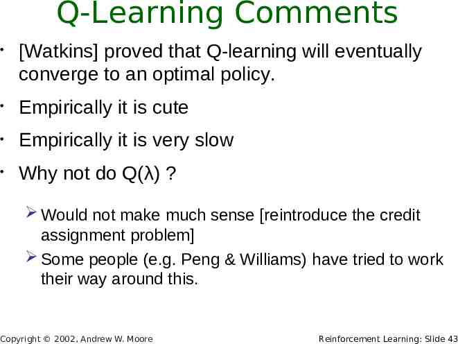
Q-Learning Comments [Watkins] proved that Q-learning will eventually converge to an optimal policy. Empirically it is cute Empirically it is very slow Why not do Q(λ) ? Would not make much sense [reintroduce the credit assignment problem] Some people (e.g. Peng & Williams) have tried to work their way around this. Copyright 2002, Andrew W. Moore Reinforcement Learning: Slide 43

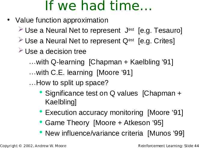
If we had time Value function approximation Use a Neural Net to represent Jest [e.g. Tesauro] Use a Neural Net to represent Qest [e.g. Crites] Use a decision tree with Q-learning [Chapman Kaelbling ’91] with C.E. learning [Moore ’91] How to split up space? Significance test on Q values [Chapman Kaelbling] Execution accuracy monitoring [Moore ’91] Game Theory [Moore Atkeson ’95] New influence/variance criteria [Munos ’99] Copyright 2002, Andrew W. Moore Reinforcement Learning: Slide 44

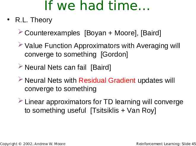
If we had time R.L. Theory Counterexamples [Boyan Moore], [Baird] Value Function Approximators with Averaging will converge to something [Gordon] Neural Nets can fail [Baird] Neural Nets with Residual Gradient updates will converge to something Linear approximators for TD learning will converge to something useful [Tsitsiklis Van Roy] Copyright 2002, Andrew W. Moore Reinforcement Learning: Slide 45

What You Should Know Supervised learning for predicting delayed rewards Certainty equivalent learning for predicting delayed rewards Model free learning (TD) for predicting delayed rewards Reinforcement Learning with MDPs: What’s the task? Why is it hard to choose actions? Q-learning (including being able to work through small simulated examples of RL) Copyright 2002, Andrew W. Moore Reinforcement Learning: Slide 46