Real time DSP Professors:  Eng. Julian Bruno  Eng. Mariano

Real time DSP Professors: Eng. Julian Bruno Eng. Mariano Llamedo Soria

Adaptive Filters

Recommended bibliography Saeed V. Vaseghi, Advanced Digital Signal Processing and Noise Reduction, Second Edition. John Wiley & Sons Ltd. Ch 3: Probabilistic Models Ch 6: Wiener Filters Ch 7: Adaptive Filters Ch 8: Linear Prediction Models Stergios Stergiopoulos, Advanced Signal Processing Handbook. CRC Press LLC, 2001 Ch 2: Adaptive Systems for Signal Process - Simon Haykin B Farhang-Boroujeny. Adaptive Filters. Theory and Applications. John Wiley & Sons. NOTE: Many images used in this presentation were extracted from the recommended bibliography .

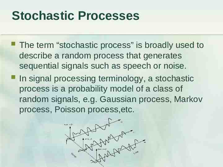
Stochastic Processes The term “stochastic process” is broadly used to describe a random process that generates sequential signals such as speech or noise. In signal processing terminology, a stochastic process is a probability model of a class of random signals, e.g. Gaussian process, Markov process, Poisson process,etc.

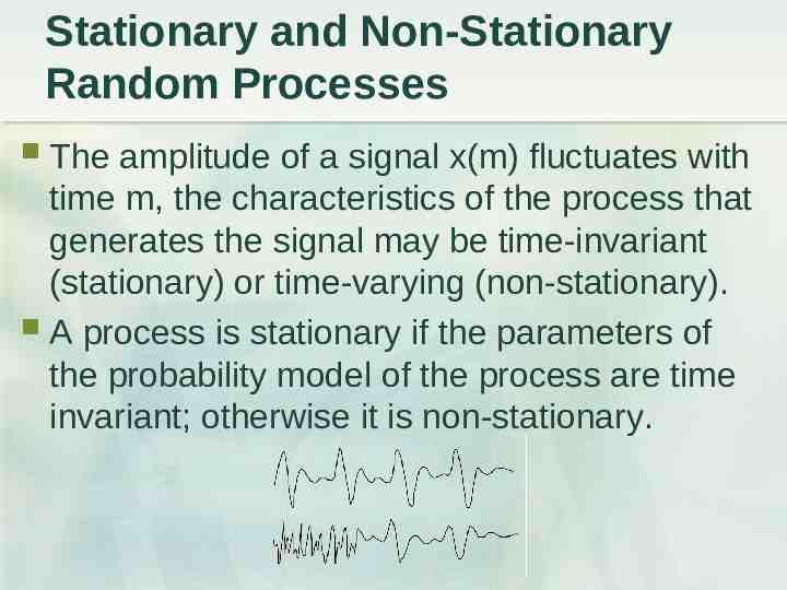
Stationary and Non-Stationary Random Processes The amplitude of a signal x(m) fluctuates with time m, the characteristics of the process that generates the signal may be time-invariant (stationary) or time-varying (non-stationary). A process is stationary if the parameters of the probability model of the process are time invariant; otherwise it is non-stationary.

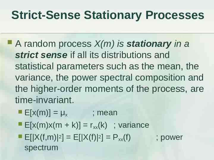
Strict-Sense Stationary Processes A random process X(m) is stationary in a strict sense if all its distributions and statistical parameters such as the mean, the variance, the power spectral composition and the higher-order moments of the process, are time-invariant. E[x(m)] μx ; mean E[x(m)x(m k)] rxx(k) ; variance E[ X(f,m) 2] E[ X(f) 2] Pxx(f) spectrum ; power

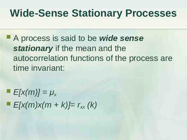
Wide-Sense Stationary Processes A process is said to be wide sense stationary if the mean and the autocorrelation functions of the process are time invariant: E[x(m)] μx E[x(m)x(m k)] rxx (k)

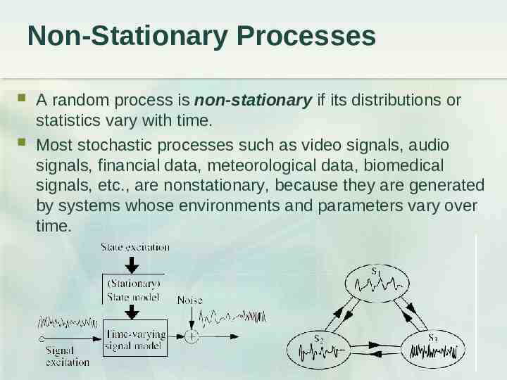
Non-Stationary Processes A random process is non-stationary if its distributions or statistics vary with time. Most stochastic processes such as video signals, audio signals, financial data, meteorological data, biomedical signals, etc., are nonstationary, because they are generated by systems whose environments and parameters vary over time.

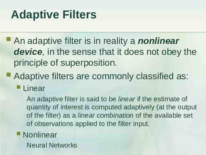
Adaptive Filters An adaptive filter is in reality a nonlinear device, in the sense that it does not obey the principle of superposition. Adaptive filters are commonly classified as: Linear An adaptive filter is said to be linear if the estimate of quantity of interest is computed adaptively (at the output of the filter) as a linear combination of the available set of observations applied to the filter input. Nonlinear Neural Networks

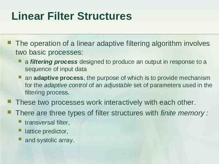
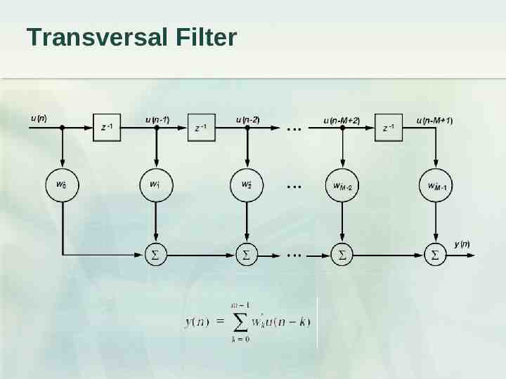
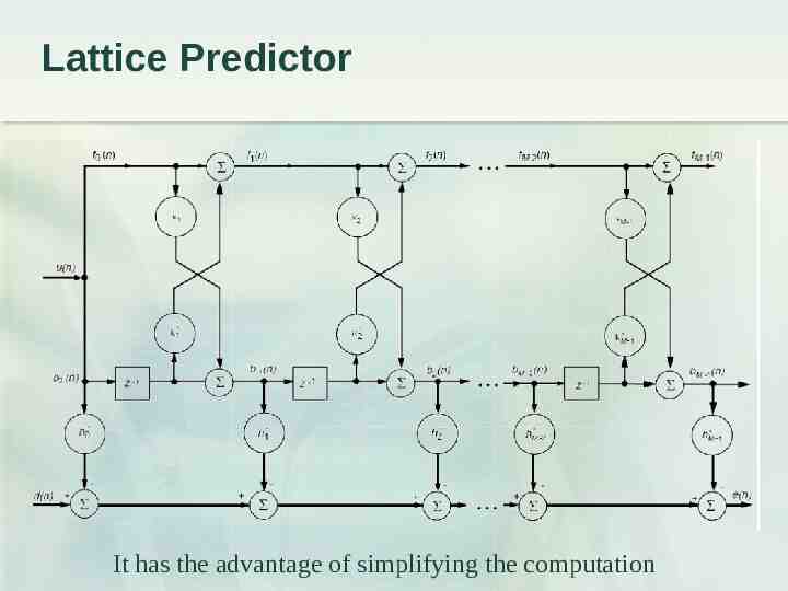
Linear Filter Structures The operation of a linear adaptive filtering algorithm involves two basic processes: a filtering process designed to produce an output in response to a sequence of input data an adaptive process, the purpose of which is to provide mechanism for the adaptive control of an adjustable set of parameters used in the filtering process. These two processes work interactively with each other. There are three types of filter structures with finite memory : transversal filter, lattice predictor, and systolic array.

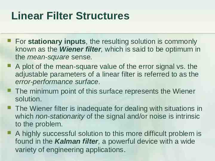
Linear Filter Structures For stationary inputs, the resulting solution is commonly known as the Wiener filter, which is said to be optimum in the mean-square sense. A plot of the mean-square value of the error signal vs. the adjustable parameters of a linear filter is referred to as the error-performance surface. The minimum point of this surface represents the Wiener solution. The Wiener filter is inadequate for dealing with situations in which non-stationarity of the signal and/or noise is intrinsic to the problem. A highly successful solution to this more difficult problem is found in the Kalman filter, a powerful device with a wide variety of engineering applications.

Transversal Filter

Lattice Predictor It has the advantage of simplifying the computation

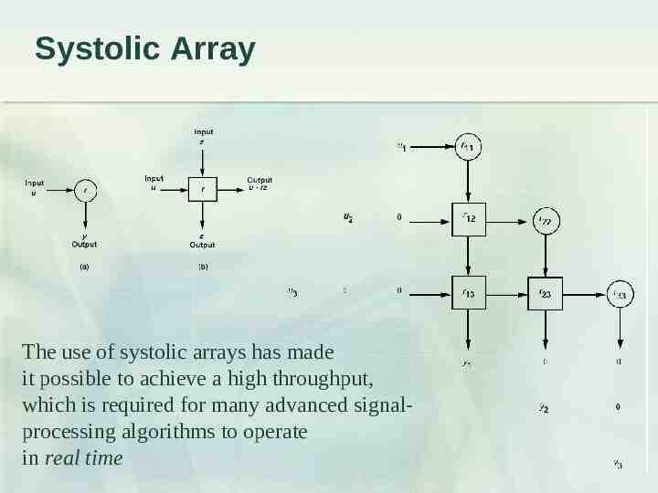
Systolic Array The use of systolic arrays has made it possible to achieve a high throughput, which is required for many advanced signalprocessing algorithms to operate in real time

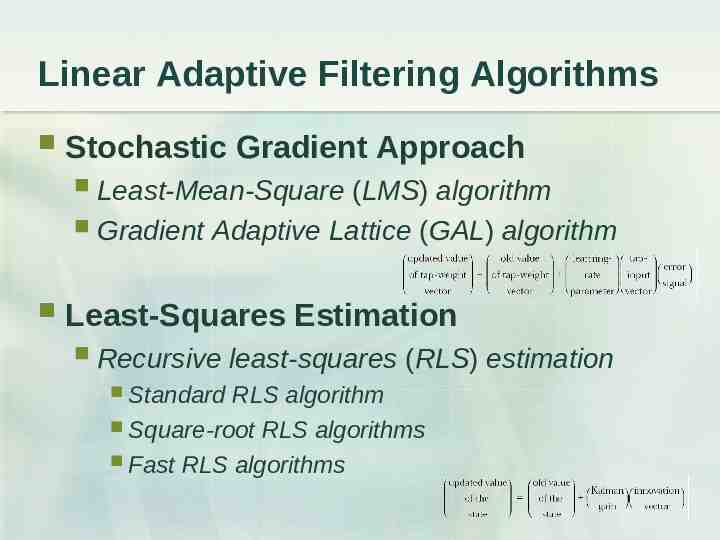
Linear Adaptive Filtering Algorithms Stochastic Gradient Approach Least-Mean-Square (LMS) algorithm Gradient Adaptive Lattice (GAL) algorithm Least-Squares Estimation Recursive least-squares (RLS) estimation Standard RLS algorithm Square-root RLS algorithms Fast RLS algorithms

Wiener Filters The design of a Wiener filter requires a priori information about the statistics of the data to be processed. The filter is optimum only when the statistical characteristics of the input data match the a priori information on which the design of the filter is based. When this information is not known completely, however, it may not be possible to design the Wiener filter or else the design may no longer be optimum.

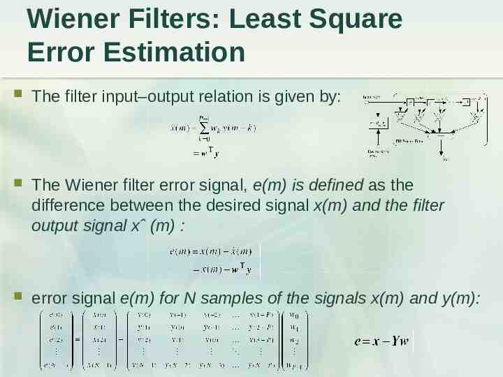
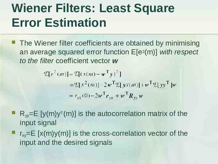
Wiener Filters: Least Square Error Estimation The filter input–output relation is given by: The Wiener filter error signal, e(m) is defined as the difference between the desired signal x(m) and the filter output signal xˆ (m) : error signal e(m) for N samples of the signals x(m) and y(m):

Wiener Filters: Least Square Error Estimation The Wiener filter coefficients are obtained by minimising an average squared error function E[e2(m)] with respect to the filter coefficient vector w Ryy E [y(m)yT(m)] is the autocorrelation matrix of the input signal rxy E [x(m)y(m)] is the cross-correlation vector of the input and the desired signals

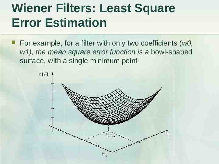
Wiener Filters: Least Square Error Estimation For example, for a filter with only two coefficients (w0, w1), the mean square error function is a bowl-shaped surface, with a single minimum point

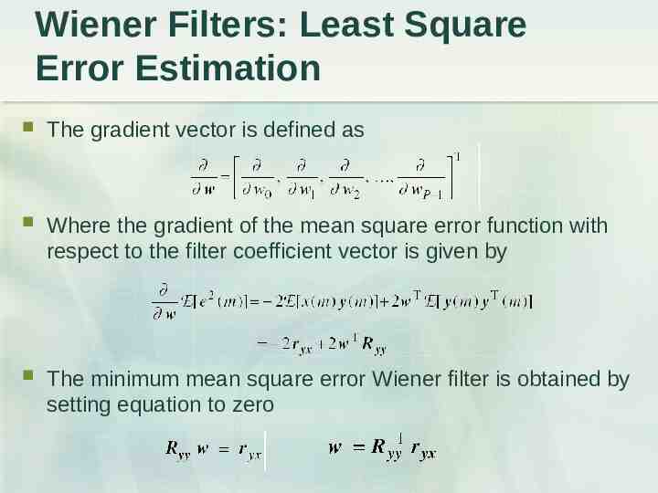
Wiener Filters: Least Square Error Estimation The gradient vector is defined as Where the gradient of the mean square error function with respect to the filter coefficient vector is given by The minimum mean square error Wiener filter is obtained by setting equation to zero

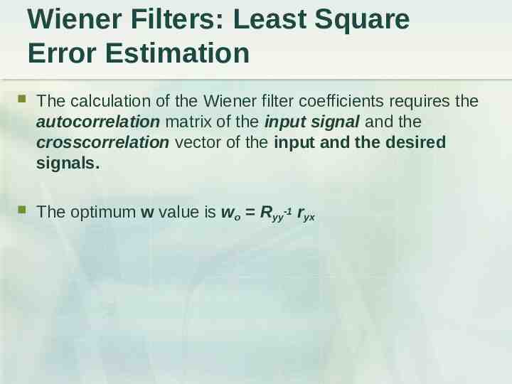
Wiener Filters: Least Square Error Estimation The calculation of the Wiener filter coefficients requires the autocorrelation matrix of the input signal and the crosscorrelation vector of the input and the desired signals. The optimum w value is wo Ryy-1 ryx

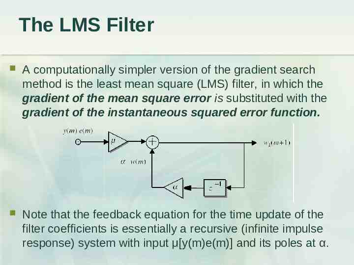
The LMS Filter A computationally simpler version of the gradient search method is the least mean square (LMS) filter, in which the gradient of the mean square error is substituted with the gradient of the instantaneous squared error function. Note that the feedback equation for the time update of the filter coefficients is essentially a recursive (infinite impulse response) system with input μ[y(m)e(m)] and its poles at α.

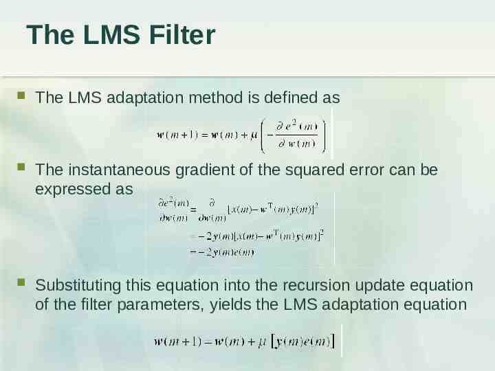
The LMS Filter The LMS adaptation method is defined as The instantaneous gradient of the squared error can be expressed as Substituting this equation into the recursion update equation of the filter parameters, yields the LMS adaptation equation

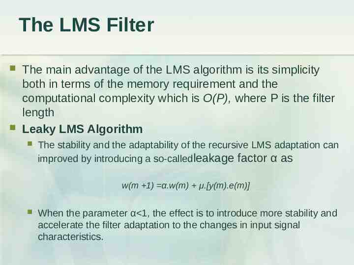
The LMS Filter The main advantage of the LMS algorithm is its simplicity both in terms of the memory requirement and the computational complexity which is O(P), where P is the filter length Leaky LMS Algorithm The stability and the adaptability of the recursive LMS adaptation can improved by introducing a so-calledleakage factor α as w(m 1) α.w(m) μ.[y(m).e(m)] When the parameter α 1, the effect is to introduce more stability and accelerate the filter adaptation to the changes in input signal characteristics.

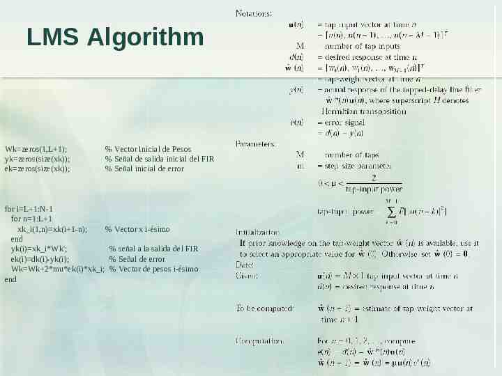
LMS Algorithm Wk zeros(1,L 1); yk zeros(size(xk)); ek zeros(size(xk)); % Vector Inicial de Pesos % Señal de salida inicial del FIR % Señal inicial de error for i L 1:N-1 for n 1:L 1 xk i(1,n) xk(i 1-n); % Vector x i-ésimo end yk(i) xk i*Wk'; % señal a la salida del FIR ek(i) dk(i)-yk(i); % Señal de error Wk Wk 2*mu*ek(i)*xk i; % Vector de pesos i-ésimo end

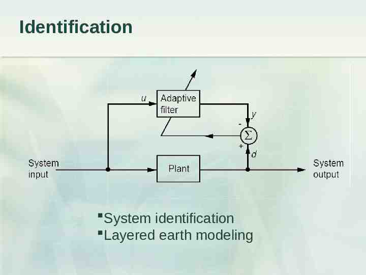
Identification System identification Layered earth modeling

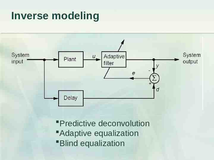
Inverse modeling Predictive deconvolution Adaptive equalization Blind equalization

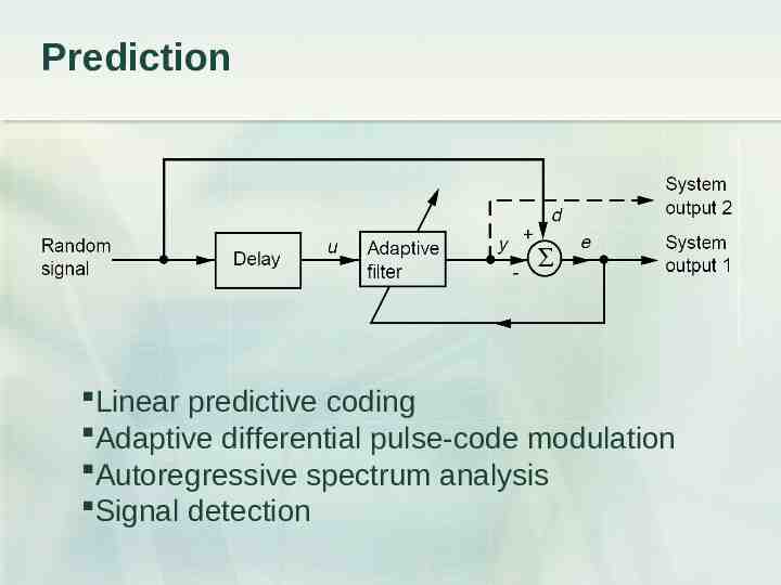
Prediction Linear predictive coding Adaptive differential pulse-code modulation Autoregressive spectrum analysis Signal detection

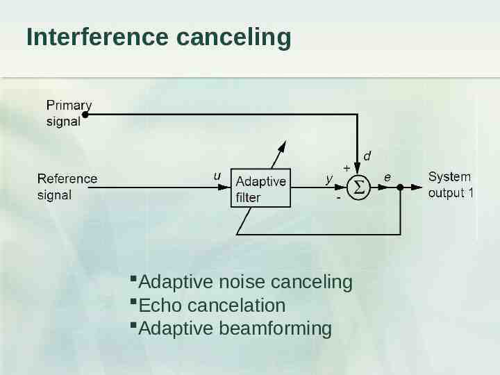
Interference canceling Adaptive noise canceling Echo cancelation Adaptive beamforming