Probability Review Thursday Sep 13

Probability Review Thursday Sep 13

Probability Review Events and Event spaces Random variables Joint probability distributions Marginalization, conditioning, chain rule, Bayes Rule, law of total probability, etc. Structural properties Independence, conditional independence Mean and Variance The big picture Examples

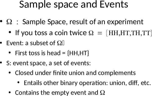
Sample space and Events Sample Space, result of an experiment If you toss a coin twice Event: a subset of First toss is head {HH,HT} S: event space, a set of events Closed under finite union and complements Entails other binary operation: union, diff, etc. Contains the empty event and

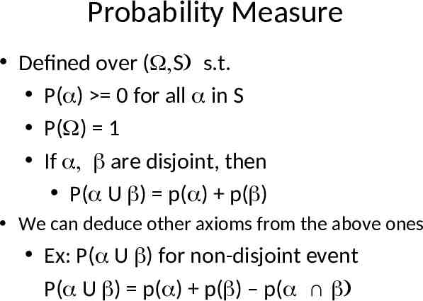
Probability Measure Defined over ( S s.t. P( ) 0 for all in S P( ) 1 If are disjoint, then P( U ) p( ) p( ) We can deduce other axioms from the above ones Ex: P( U ) for non-disjoint event P( U ) p( ) p( ) – p(

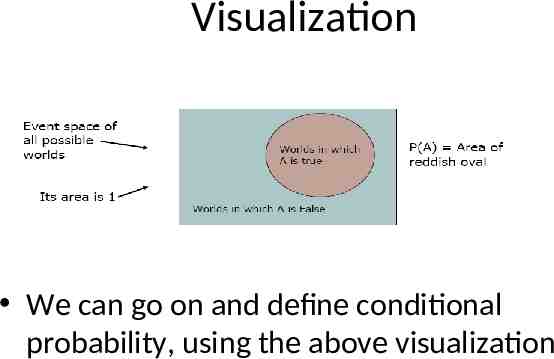
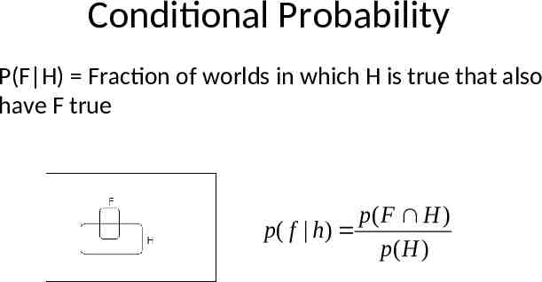
Visualization We can go on and define conditional probability, using the above visualization

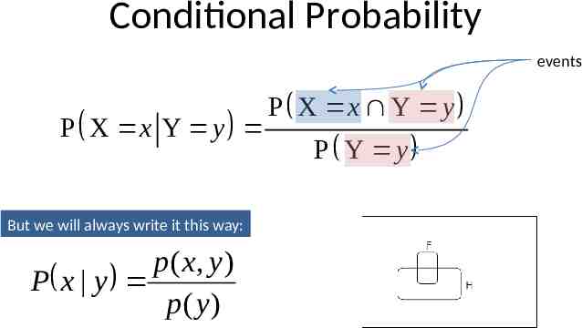
Conditional Probability P(F H) Fraction of worlds in which H is true that also have F true p( F H ) p ( f h) p( H )

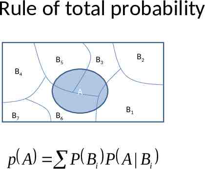
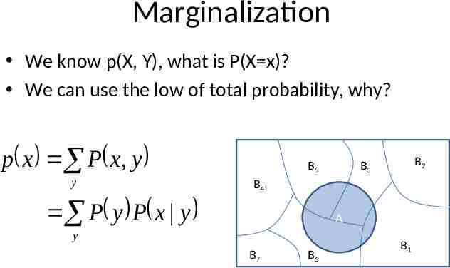
Rule of total probability B5 B2 B3 B4 A B7 B6 B1 p A P Bi P A Bi

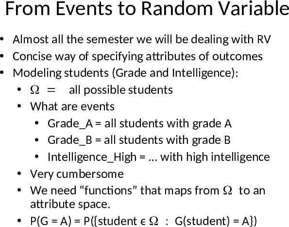
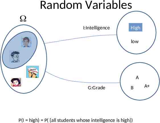
From Events to Random Variable Almost all the semester we will be dealing with RV Concise way of specifying attributes of outcomes Modeling students (Grade and Intelligence): all possible students What are events Grade A all students with grade A Grade B all students with grade B Intelligence High with high intelligence Very cumbersome We need “functions” that maps from to an attribute space. P(G A) P({student ϵ G(student) A})

Random Variables I:Intelligence High low A G:Grade B P(I high) P( {all students whose intelligence is high}) A

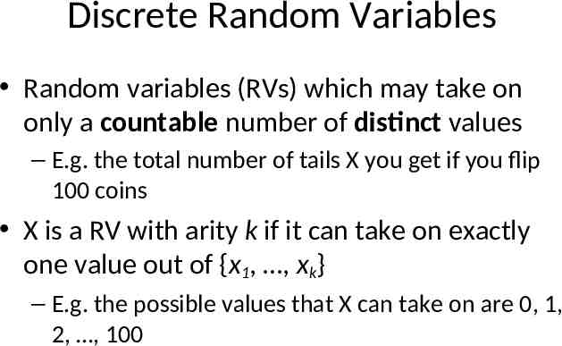
Discrete Random Variables Random variables (RVs) which may take on only a countable number of distinct values – E.g. the total number of tails X you get if you flip 100 coins X is a RV with arity k if it can take on exactly one value out of {x1, , xk} – E.g. the possible values that X can take on are 0, 1, 2, , 100

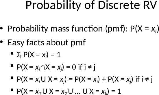
Probability of Discrete RV Probability mass function (pmf): P(X xi) Easy facts about pmf Σi P(X xi) 1 P(X xi X xj) 0 if i j P(X xi U X xj) P(X xi) P(X xj) if i j P(X x1 U X x2 U U X xk) 1

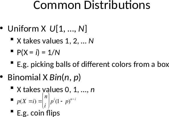
Common Distributions Uniform X U[1, , N] X takes values 1, 2, N P(X i) 1/N E.g. picking balls of different colors from a box Binomial X Bin(n, p) X takes values 0, 1, , n n i p(X i) p (1 p)n i i E.g. coin flips

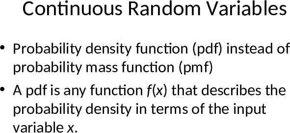
Continuous Random Variables Probability density function (pdf) instead of probability mass function (pmf) A pdf is any function f(x) that describes the probability density in terms of the input variable x.

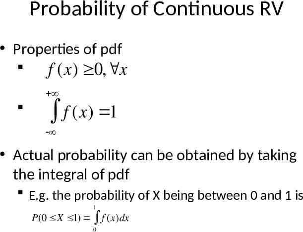
Probability of Continuous RV Properties of pdf f (x) 0, x f (x) 1 Actual probability can be obtained by taking the integral of pdf E.g. the probability of X being between 0 and 1 is 1 P(0 X 1) f (x)dx 0

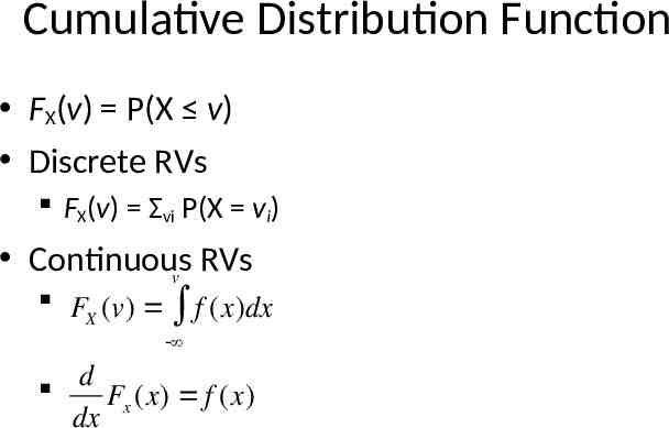
Cumulative Distribution Function FX(v) P(X v) Discrete RVs FX(v) Σvi P(X vi) Continuous RVs v FX (v) f (x)dx d Fx (x) f (x) dx

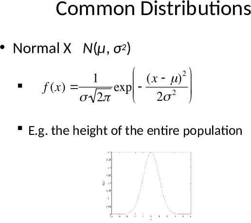
Common Distributions Normal X N(μ, σ2) (x ) 2 1 f (x) exp 2 2 2 E.g. the height of the entire population

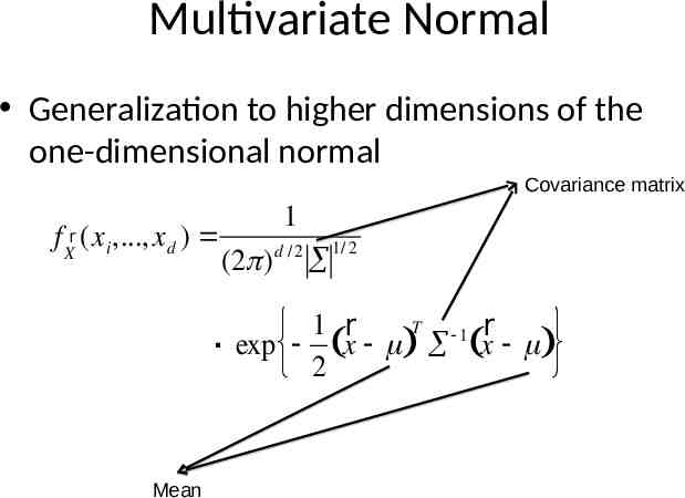
Multivariate Normal Generalization to higher dimensions of the one-dimensional normal Covariance matrix 1 f Xr (x i ,., x d ) 1/ 2 d /2 (2 ) . exp 1 xr T 1 xr 2 Mean

Probability Review Events and Event spaces Random variables Joint probability distributions Marginalization, conditioning, chain rule, Bayes Rule, law of total probability, etc. Structural properties Independence, conditional independence Mean and Variance The big picture Examples

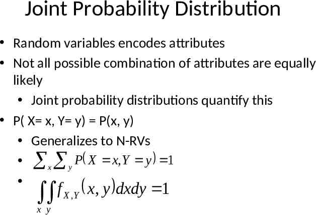
Joint Probability Distribution Random variables encodes attributes Not all possible combination of attributes are equally likely Joint probability distributions quantify this P( X x, Y y) P(x, y) Generalizes to N-RVs x y P X x, Y y 1 f x, y dxdy 1 X ,Y x y

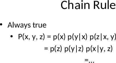
Chain Rule Always true P(x, y, z) p(x) p(y x) p(z x, y) p(z) p(y z) p(x y, z)

Conditional Probability events P X x Y y But we will always write it this way: p ( x, y ) P x y p( y ) P X x Y y P Y y

Marginalization We know p(X, Y), what is P(X x)? We can use the low of total probability, why? p x P x, y y B5 B2 B3 B4 P y P x y A y B7 B6 B1

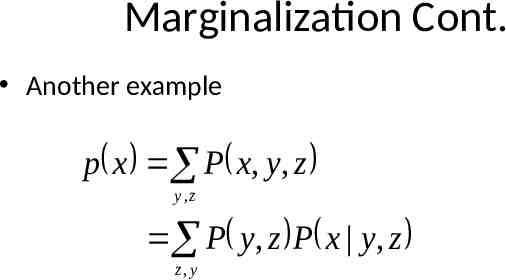
Marginalization Cont. Another example p x P x, y, z y,z P y, z P x y, z z,y

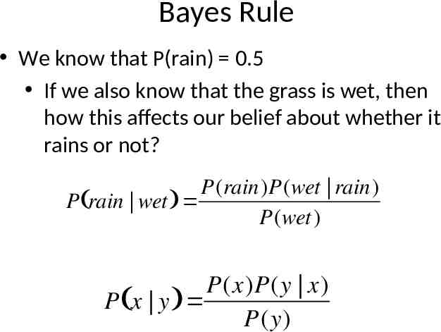
Bayes Rule We know that P(rain) 0.5 If we also know that the grass is wet, then how this affects our belief about whether it rains or not? P(rain)P(wet rain) P rain wet P(wet) P(x)P(y x) P x y P(y)

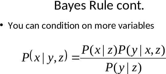
Bayes Rule cont. You can condition on more variables P ( x z ) P ( y x, z ) P x y, z P( y z )

Probability Review Events and Event spaces Random variables Joint probability distributions Marginalization, conditioning, chain rule, Bayes Rule, law of total probability, etc. Structural properties Independence, conditional independence Mean and Variance The big picture Examples

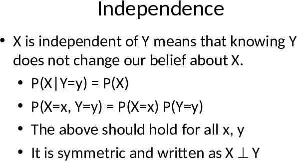
Independence X is independent of Y means that knowing Y does not change our belief about X. P(X Y y) P(X) P(X x, Y y) P(X x) P(Y y) The above should hold for all x, y It is symmetric and written as X Y

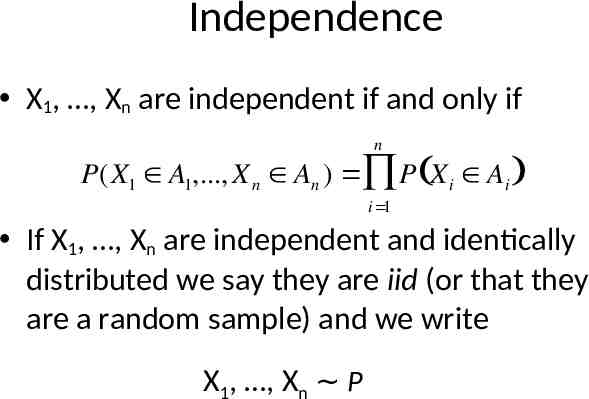
Independence X1, , Xn are independent if and only if n P(X1 A1,., X n An ) P X i Ai i 1 If X1, , Xn are independent and identically distributed we say they are iid (or that they are a random sample) and we write X1, , Xn P

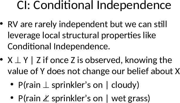
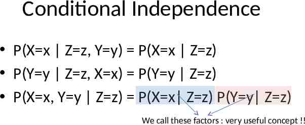
CI: Conditional Independence RV are rarely independent but we can still leverage local structural properties like Conditional Independence. X Y Z if once Z is observed, knowing the value of Y does not change our belief about X P(rain sprinkler’s on cloudy) P(rain sprinkler’s on wet grass)

Conditional Independence P(X x Z z, Y y) P(X x Z z) P(Y y Z z, X x) P(Y y Z z) P(X x, Y y Z z) P(X x Z z) P(Y y Z z) We call these factors : very useful concept !!

Probability Review Events and Event spaces Random variables Joint probability distributions Marginalization, conditioning, chain rule, Bayes Rule, law of total probability, etc. Structural properties Independence, conditional independence Mean and Variance The big picture Examples

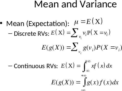
Mean and Variance Mean (Expectation): E X – Discrete RVs: E X v vi P X vi i E(g(X)) v g(v i )P(X v i ) i – Continuous RVs: E X xf x dx E(g(X)) g(x) f (x)dx

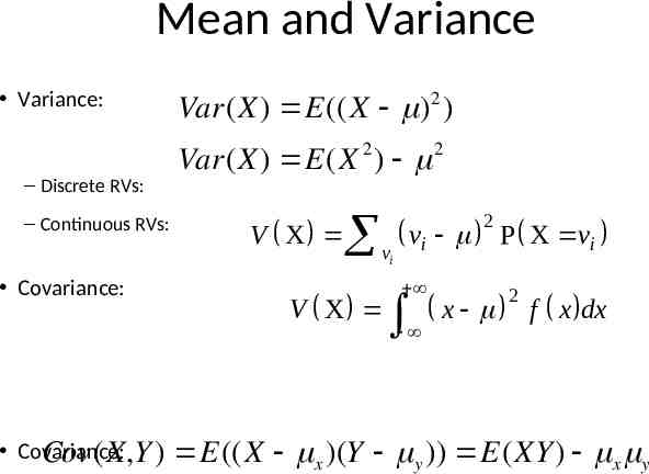
Mean and Variance Variance: – Discrete RVs: – Continuous RVs: Covariance: Covariance: Cov(X,Y ) 2 Var(X) E((X ) ) Var(X) E(X 2 ) 2 V X 2 vi V X vi P X vi x 2 f x dx E((X x )(Y y )) E (XY) x y

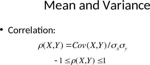
Mean and Variance Correlation: (X,Y ) Cov(X,Y ) / x y 1 (X,Y ) 1

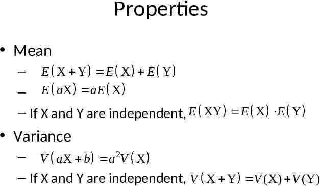
Properties Mean – E X Y E X E Y – E aX aE X – If X and Y are independent, E XY E X E Y Variance – V aX b a 2V X – If X and Y are independent, V X Y V (X) V (Y)

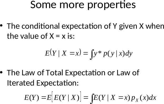
Some more properties The conditional expectation of Y given X when the value of X x is: E Y X x y * p( y x)dy The Law of Total Expectation or Law of Iterated Expectation: E (Y ) E E (Y X ) E (Y X x) p X ( x)dx

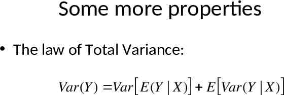
Some more properties The law of Total Variance: Var(Y ) Var E(Y X ) E Var(Y X)

Probability Review Events and Event spaces Random variables Joint probability distributions Marginalization, conditioning, chain rule, Bayes Rule, law of total probability, etc. Structural properties Independence, conditional independence Mean and Variance The big picture Examples

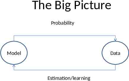
The Big Picture Probability Model Data Estimation/learning

Statistical Inference Given observations from a model – What (conditional) independence assumptions hold? Structure learning – If you know the family of the model (ex, multinomial), What are the value of the parameters: MLE, Bayesian estimation. Parameter learning

Probability Review Events and Event spaces Random variables Joint probability distributions Marginalization, conditioning, chain rule, Bayes Rule, law of total probability, etc. Structural properties Independence, conditional independence Mean and Variance The big picture Examples

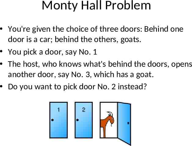
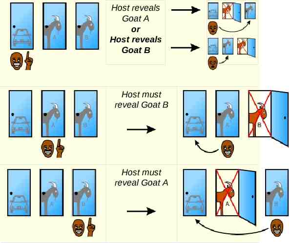
Monty Hall Problem You're given the choice of three doors: Behind one door is a car; behind the others, goats. You pick a door, say No. 1 The host, who knows what's behind the doors, opens another door, say No. 3, which has a goat. Do you want to pick door No. 2 instead?

Host reveals Goat A or Host reveals Goat B Host must reveal Goat B Host must reveal Goat A

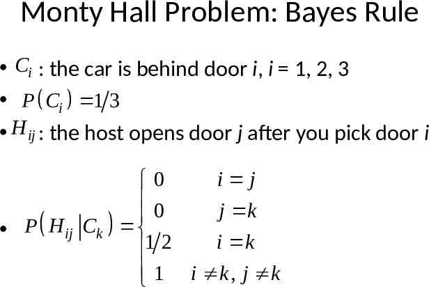
Monty Hall Problem: Bayes Rule Ci : the car is behind door i, i 1, 2, 3 P Ci 1 3 H ij : the host opens door j after you pick door i P H ij Ck i j 0 0 j k i k 1 2 1 i k , j k

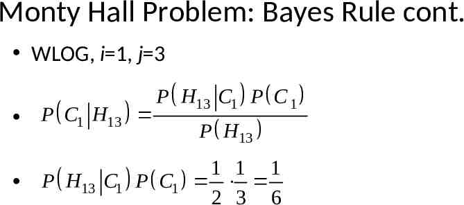
Monty Hall Problem: Bayes Rule cont. WLOG, i 1, j 3 P C1 H13 P H13 P H13 C1 P C 1 P H13 1 1 1 C1 P C1 2 3 6

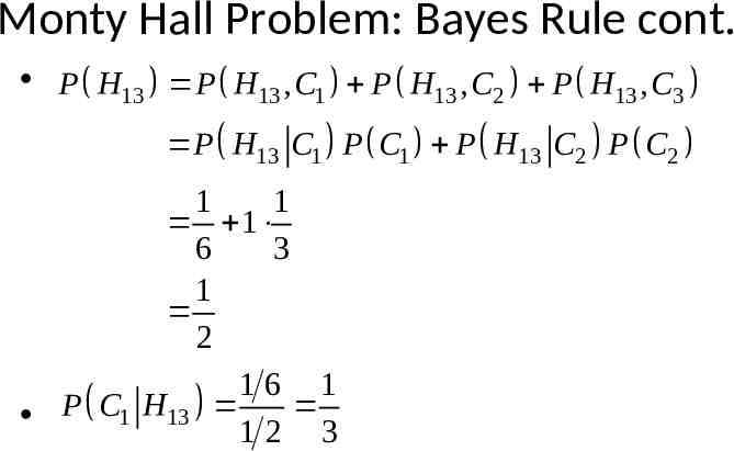
Monty Hall Problem: Bayes Rule cont. P H13 P H13 , C1 P H13 , C2 P H13 , C3 P H13 C1 P C1 P H13 C2 P C2 1 1 1 6 3 1 2 16 1 P C1 H13 1 2 3

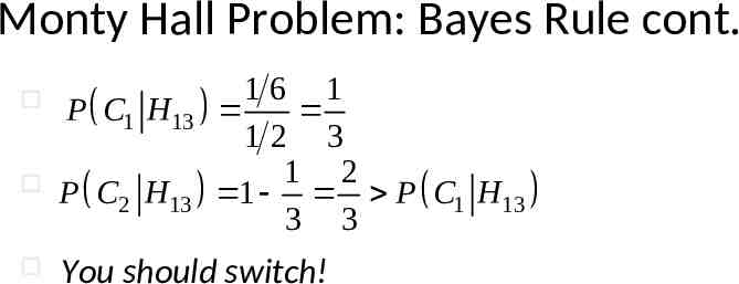
Monty Hall Problem: Bayes Rule cont. 16 1 P C1 H13 12 3 1 2 P C2 H13 1 P C1 H13 3 3 You should switch!

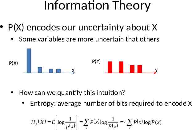
Information Theory P(X) encodes our uncertainty about X Some variables are more uncertain that others P(Y) P(X) X Y How can we quantify this intuition? Entropy: average number of bits required to encode X 1 1 H P X E log P x log P x log P( x) p x P x x x

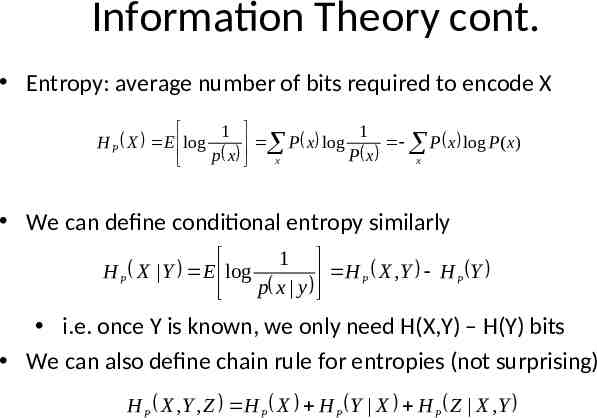
Information Theory cont. Entropy: average number of bits required to encode X 1 1 H P X E log P x log P x log P ( x) p x P x x x We can define conditional entropy similarly 1 H P X Y E log H P X , Y H P Y p x y i.e. once Y is known, we only need H(X,Y) – H(Y) bits We can also define chain rule for entropies (not surprising) H P X , Y , Z H P X H P Y X H P Z X , Y

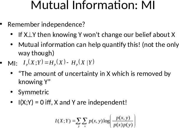
Mutual Information: MI Remember independence? If X Y then knowing Y won’t change our belief about X Mutual information can help quantify this! (not the only way though) MI: I P X ;Y H P X H P X Y “The amount of uncertainty in X which is removed by knowing Y” Symmetric I(X;Y) 0 iff, X and Y are independent! p ( x, y ) I ( X ; Y ) p( x, y ) log y x p( x) p( y )

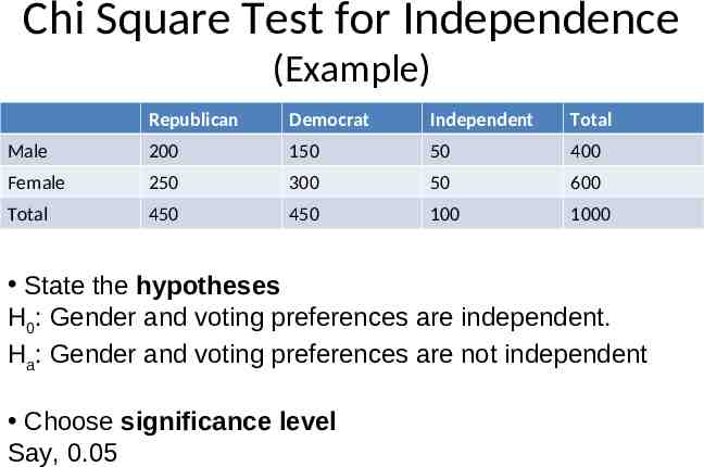
Chi Square Test for Independence (Example) Republican Democrat Independent Total Male 200 150 50 400 Female 250 300 50 600 Total 450 450 100 1000 State the hypotheses H0: Gender and voting preferences are independent. Ha: Gender and voting preferences are not independent Choose significance level Say, 0.05

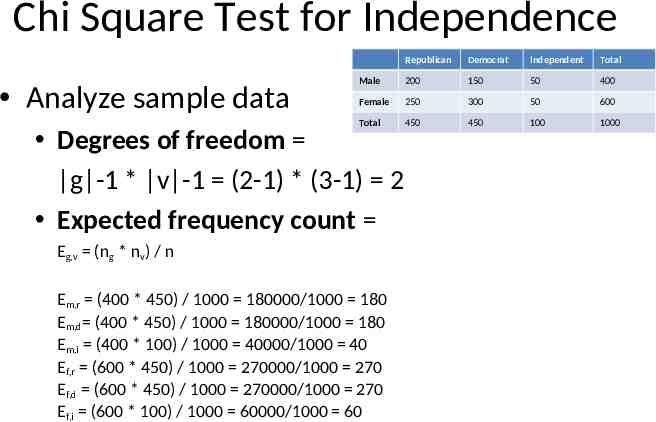
Chi Square Test for Independence Analyze sample data Republican Democrat Independent Total Male 200 150 50 400 Female 250 300 50 600 Total 450 450 100 1000 Degrees of freedom g -1 * v -1 (2-1) * (3-1) 2 Expected frequency count Eg,v (ng * nv) / n Em,r (400 * 450) / 1000 180000/1000 180 Em,d (400 * 450) / 1000 180000/1000 180 Em,i (400 * 100) / 1000 40000/1000 40 Ef,r (600 * 450) / 1000 270000/1000 270 Ef,d (600 * 450) / 1000 270000/1000 270 Ef,i (600 * 100) / 1000 60000/1000 60

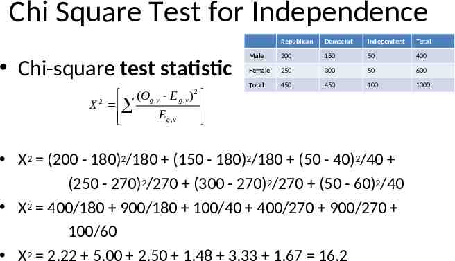
Chi Square Test for Independence Chi-square test statistic (Og ,v E g ,v ) X E g ,v 2 2 Republican Democrat Independent Total Male 200 150 50 400 Female 250 300 50 600 Total 450 450 100 1000 Χ2 (200 - 180)2/180 (150 - 180)2/180 (50 - 40)2/40 (250 - 270)2/270 (300 - 270)2/270 (50 - 60)2/40 Χ2 400/180 900/180 100/40 400/270 900/270 100/60 Χ2 2.22 5.00 2.50 1.48 3.33 1.67 16.2

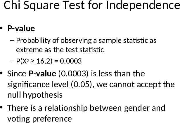
Chi Square Test for Independence P-value – Probability of observing a sample statistic as extreme as the test statistic – P(X2 16.2) 0.0003 Since P-value (0.0003) is less than the significance level (0.05), we cannot accept the null hypothesis There is a relationship between gender and voting preference

Acknowledgment Carlos Guestrin recitation slides: http://www.cs.cmu.edu/ guestrin/Class/10708/recitations/r1/Probability and St atistics Review.ppt Andrew Moore Tutorial: http://www.autonlab.org/tutorials/prob.html Monty hall problem: http://en.wikipedia.org/wiki/Monty Hall problem http://www.cs.cmu.edu/ guestrin/Class/10701-F07/recitation schedule.html Chi-square test for independence http://stattrek.com/chi-square-test/independence.aspx