Performance Optimization for the Origin 2000

Performance Optimization for the Origin 2000 http://www.cs.utk.edu/ mucci/MPPopt.html Kevin London ([email protected]) Philip Mucci ([email protected]) University of Tennessee, Knoxville Army Research Laboratory, Aug. 31 - Sep. 2

SGI Optimization Tutorial Day 1

Getting Started First logon to an origin 2000. Today we will be using eckert. Copy the tutorials to your home area. They can be found in: london/arl tutorial You can copy all the necessary files by: Cp -rf london/arl tutorial /.

Getting Started (Continued) For todays tutorial we will be using the files in /ARL TUTORIAL/DAY1 We will be using some performance analysis tools to look at fft code written in MPI.

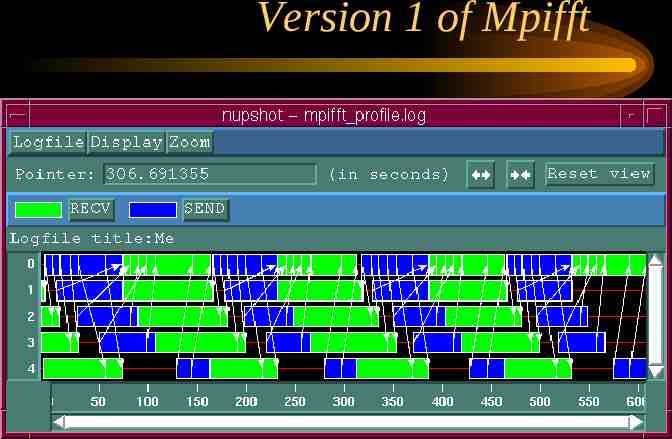
Version 1 of Mpifft

Version 2 of Mpifft

Version 3 of Mpifft

perfex perfex is useful for a first pass on your code Today run perfex on mpifft the following way: – mpirun -np 5 perfex -mp -x -y -a mpifft

Speedshop Tools ssusage -- allows you to collect information about your machines resources ssrun -- this is the command to run experiments on a program to collect performance data prof -- analyzes the performance data you have recorded using ssrun

Speedshop Experiment Types Statistical PC sampling with pcsamp experiments Statistical hardware counter sampling with hwc experiments. (On R10000 systems with built-in hardware counters) Statistical call stack profiling with usertime Basic block counting with ideal

Speedshop Experiment Types Floating point exception trace with fpe

Using Speedshop Tools for Performance Analysis The general steps for a performance analysis cycle are: Build the application Run experiments on the application to collect performance data Examine the performance data Generate an improved version of the program Repeat as needed

Using ssusage on Your Program Run your program with ssusage: – ssusage program name This allows you to identify high user CPU time, high system CPU time, high I/O time, and a high degree of paging With this information you can then decide on which experiments to run for further study

ssusage (Continued) In this tutorial ssusage will be called like the following: – ssusage mpirun -np 5 mpifft The output will look something like this: – 38.31 real, 0.02 user, 0.08 sys, 0 majf, 117 minf, 0 sw, 0 rb, 0 wb, 172 vcx, 1 icx – Real-time, user-cpu time, system-cpu time, major page faults (those causing physical I/O), minor page faults (those requiring mapping only), swaps, physical blocks read and written, voluntary context switches and involuntary context switches.

Using ssrun on Your Program To collect performance data, call ssrun as follows: – ssrun flags exp type prog name prog args – Flags are one or more valid flags – Exp type experiment name – Prog name executable name – Prog args any arguments to the executable

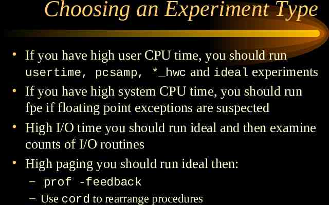
Choosing an Experiment Type If you have high user CPU time, you should run usertime, pcsamp, * hwc and ideal experiments If you have high system CPU time, you should run fpe if floating point exceptions are suspected High I/O time you should run ideal and then examine counts of I/O routines High paging you should run ideal then: – prof -feedback – Use cord to rearrange procedures

Running Experiments on a MPI Program Running experiments on MPI programs is a little different You need to setup a script to run experiments with them – #!/Bin/sh – Ssrun -usertime mpifft You then run the script by: – mpirun -np 5 script

Experiments That We Will Run for the Tutorial. usertime fpcsamp ideal dsc hwc -- secondary data cache misses tlb hwc -- TLB misses

usertime This experiment is already setup in runmpifft in the v[1-3] directories To run the experiment use: – mpirun -np 5 runmpifft This will give you 6 files in the directory: mpifft.usertime.? To look at the results use: – prof mpifft.usertime.?

usertime (Continued) Example output: Cpu : r10000 Fpu : r10010 Clock : 195.0mhz Number of cpus : 32 Index %samples self descendents total name [1] 95.7% 0.00 17.82 594 fork child handle [2] 78.7% 0.00 14.67 489 slave main [3] 53.6% 0.72 9.27 333 slave receive data %Samples is the total percentage of samples take in this function or its descendants. Self, and descendants are the time spent in that function and its descendants as determined by the number of samples in that function * the sample interval. Total is the number of samples.

fpcsamp To run this experiment you need to edit the runmpifft script and change the line: – ssun -usertime mpifft – ssrun -fpcsamp mpifft to: Once again this will give you 6 files in your directory: – mpifft.fpcsamp.? To look at the results use: – prof mpifft.fpcsamp.?

fpcsamp (Continued) Example output: Samples time CPU FPU clock n-cpu s-interval countsize 30990 30.99s r10000 r10010 195.0mhz 32 1.0ms 2(bytes) Each sample covers 4 bytes for every 1.0 ms ( 0.00% of 30.9900s) ----------------------------------------------------------------------------------------Samples time(%) cum time(%) procedure (dso:file) 4089 4.09s( 13.2) 4.09s( 13.2) one fft (mpifft:/home/army/london/eckert/arl tutorial/day1/v1/slave.C) 3669 3.67s( 11.8) 7.76s( 25.0) mpi sgi progress(/usr/lib32/libmpi.So:/xlvll/array/array 3.0/work/mpi/ lib/libmpi/libmpi n32 m4/adi/progress.C)

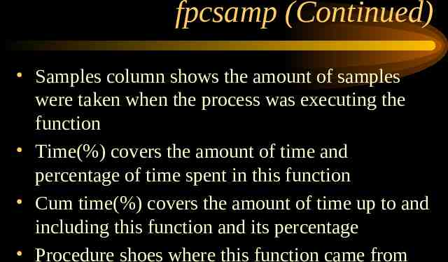
fpcsamp (Continued) Samples column shows the amount of samples were taken when the process was executing the function Time(%) covers the amount of time and percentage of time spent in this function Cum time(%) covers the amount of time up to and including this function and its percentage Procedure shoes where this function came from

ideal To run this experiment you need to edit the runmpifft script and change the line to: – ssrun -ideal mpifft This will leave 13 files in your directory – 6 mpifft.ideal.? – spifft.pixie – 6 lib*.pixn32 files for ex. libmpi.so.pixn32 To view the results type: – prof mpifft.ideal.?

ideal (Continued) Example output: 2332123106: total number of cycles 11.95961s: total execution time 2924993455: total number of instructions executed 0.797: ratio of cycles / instruction 195: clock rate in mhz R10000: target processor modeled Cycles(%) cum % secs instrns calls procedure(dso:file) 901180416(38.64) 38.64 4.62 1085714432 2048 mpifft.Pixie:/home/army/london/eckert/arl tutorial/day1/v1/slave.C)

ideal (Continued) Cycles (%) reports the number and procedure Cum% column shows the cumulative percentage of calls Secs column shows the number of seconds spent in the procedure Instrns column shows the number of instructions executed for the procedure Calls column reports the number of calls to the procedure Procedure column shows you which function and where it is coming from.

Secondary Data Cache Misses (dsc hwc) To run this experiment you need to change the line in the runmpifft script to: – ssrun -dsc hwc mpifft This will leave 6 files in your directory: – 6 mpifft.fdsc hwc.? To view the results type: – prof mpifft.dsc hwc.?

Secondary Data Cache Misses (dsc hwc) (Continued) Example output: Counter : sec cache D misses Counter overflow value : 131 Total number of ovfls : 38925 Cpu : r10000 Fpu : r10010 Clock : 195.0 mhz Number of cpus : 32 -----------------------------------------------------------------------------------------Overflows(%) cum overflows(%) procedure (dso:file) 11411( 29.3) 11411( 29.3) memcpy (/usr/lib32/libc.So.1:/xlv21/patches/3108/work/irix/lib/libx/libc n32 m4/strings/ bcopy.S)

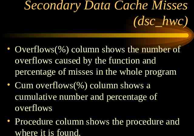
Secondary Data Cache Misses (dsc hwc) Overflows(%) column shows the number of overflows caused by the function and percentage of misses in the whole program Cum overflows(%) column shows a cumulative number and percentage of overflows Procedure column shows the procedure and where it is found.

Translation Lookaside Buffer Misses (tlb hwc) To run this experiment you need to change the line in the runmpifft script to: – ssrun -tlb hwc mpifft This will leave 6 files in your directory: – 6 mpifft.tlb hwc.? To look at the results use: – prof mpifft.tlb hwc.?

Translation Lookaside Buffer Misses (tlb hwc) Example output: Counter : TLB misses Counter overflow value : 257 Total number of ovfls : 120 Cpu : r10000 Fpu : r10010 Clock : 195.0 mhz Number of cpus : 32 -----------------------------------------------------------------------------------------Overflows(%) cum overflows(%) procedure (dso:file) 25( 20.8) 25( 20.8) mpi sgi barsync (/usr/lib32/libmpi.So:/xlvll/array/array 3.0/work/mpi/lib/libmpi/libmpi n32 m4/ sgimp/barsync.C)

SGI Optimization Tutorial Day 2

More Info on Tools http://www.cs.utk.edu/ browne/perftools-review http://www.nhse.org/ptlib

Getting the new files You need to cd into /ARL TUTORIAL/DAY1 Then cp london/ARL TUTORIAL/DAY1/make* .

Outline nupshot tutorial vampir tutorial matrix multiply tutorial

Nupshot view

nupshot nupshot is distributed with the mpich distribution. nupshot can read alog and picl-1 log files. A good way to get a quick overview of how your well the communication in your program is doing.

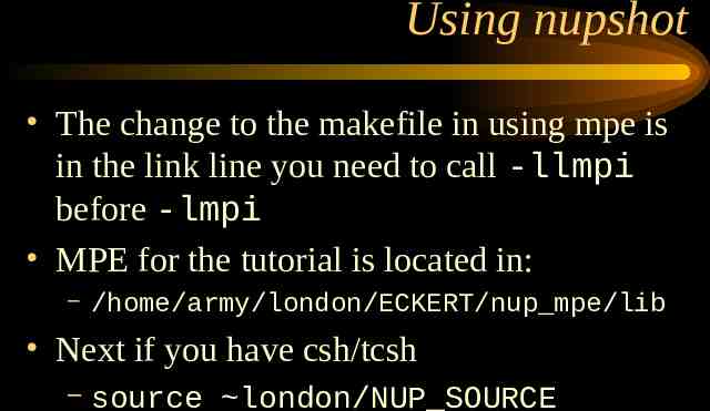
Using nupshot The change to the makefile in using mpe is in the link line you need to call -llmpi before -lmpi MPE for the tutorial is located in: – /home/army/london/ECKERT/nup mpe/lib Next if you have csh/tcsh – source london/NUP SOURCE

Using nupshot (continued) This file has the following stuff adding to your environment: – setenv TCL LIBRARY /ha/cta/unsupported/SPE/profiling/tcl7.3-tk3.6/lib – setenv TK LIBRARY /ha/cta/unsupported/SPE/profiling/tcl7.3-tk3.6/lib – set path ( path /ha/cta/unsupported/SPE/profiling/nupshot These will setup the correct TCL/TK libraries and that nupshot is in your path. Then you need to set your display and use xhost to authorize eckert to connect to your display.

Using nupshot (continued) For example: – setenv DISPLAY heat04.ha.md.us – On heat04 type xhost eckert If you don’t use csh/tcsh all the variables need to be set up by hand and you can do it this way: – DISPLAY heat04.ha.md.us – export DISPLAY

Running the example To make the example go into the DAY1 directory and type: – make clean – make This will link in the mpe profiling library and make the executables. To run the executables go into the v1, v2 and v3 directories and type: – mpirun -np 5 mpifft

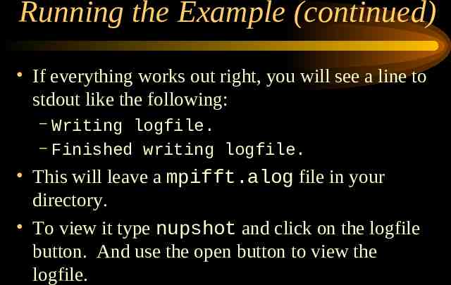
Running the Example (continued) If everything works out right, you will see a line to stdout like the following: – Writing logfile. – Finished writing logfile. This will leave a mpifft.alog file in your directory. To view it type nupshot and click on the logfile button. And use the open button to view the logfile.

Running the Example (continued) This will bring up a timeline window, you can also get a mountain range view by clicking on Display, then on configure and click on add and mountain ranges. The mountain ranges view is a histogram of the states the processors are in at any one time. If you click and hold in the timeline display on a MPI call it will tell you the start/stop time and total amount of time spent in that call.

Vampir Tutorial (Getting Started) Setup environment variables for the vampir tracing tools. – setenv PAL ROOT /home/army/london/ECKERT/vampir-trace In your makefile you need to link in the vampir library – -L/home/army/london/ECKERT/vampir-trace/lib -lVT This needs to be linked in before mpi. Then run your executable like normal.

Vampir Tutorial Creating a logfile To setup the tutorial for vampir go into the DAY1 directory and do the following: – rm make.def – ln -s make vampir.sgi make.def – make Then run the executables using – mpirun -np 5 mpifft If everything goes right you will see: – Writing logfile mpifft.bpv – Finished writing logfile.

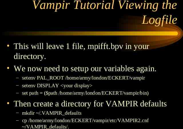
Vampir Tutorial Viewing the Logfile This will leave 1 file, mpifft.bpv in your directory. We now need to setup our variables again. – setenv PAL ROOT /home/army/london/ECKERT/vampir – setenv DISPLAY your display – set path ( path /home/army/london/ECKERT/vampir/bin) Then create a directory for VAMPIR defaults – mkdir /.VAMPIR defaults – cp /home/army/london/ECKERT/vampir/etc/VAMPIR2.cnf /VAMPIR defaults/.

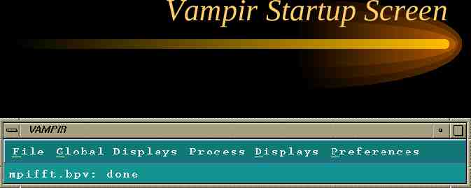
Using Vampir To start up Vampir use – vampir & From the “File” menu, select “Open Tracefile ”. A file selection box will appear. Choose mpifft.bpv We’ll start by viewing the timeline for the the entire run. From the “Global Displays” menu, select “Global Timeline”. A window with the timeline will pop up. Zoom in on a section of the timeline: Click and drag over a portion of the timeline with the left mouse button. This part will be magnified. If you zoom in close enough you will see the MPI calls.

Vampir Startup Screen

Vampir Timeline Display

Using Vampir viewing statistics for selected portion of the timeline. View process statistics for the selected portion of the timeline. From the “Global Displays” menu, select “Global Activity Chart”. A new window will open. Press the right mouse button within this window. Select “Use Timeline Portion”. Scroll the timeline, using the scroll bar at the bottom of the timeline window, and watch what happens in both displays. Press the right mouse button in the “Global Activity Chart” and select “Close”.

Vampir Global Activity Chat

Vampir, additional info on messages Obtain additional information on messages. Click on the “Global Timeline” window with the right mouse button. From the pop-up menu, select “Identify Message”. Messages are drawn as lines between processes. Click on any message with the left mouse button. A window with message information should pop up. Press the “Close” button when finished reading. To exit VAMPIR from the “File” menu select “Exit”.

Identifying a message in Vampir

Identifying messages in Vampir

Matrix-Matrix Multiply Demo These exercises are to get you familiar with some of the code optimizations that we went over early today. All of these exercises are located in the DAY2 directory.

Exercise 1 This first exercise will use a simple matrixmatrix inner product multiplication to demonstrate various optimization techniques.

Matrix-Matrix Multiplication Simple Optimization by Cache Reuse Purpose: The exercise is intended to show how the reuse of data that has been loaded into cache by some previous instruction can save time and thus increase the performance of your code. Information: Perform the matrix multiplication A A B*C using the code segment below as a template and ordering the ijk loops in to the following orders( ijk, jki, kij, and kji). In the file matmul.f, one ordering has been provided for you (ijk), as well as high performance BLAS routine dgemm which does double precision general matrix multiplication. dgemm and other routines can be obtained from Netlib. The cariables in the matmul routine (reproduced on the next page) are chosen for compatibility with the BLAS routines and have the following meanings: the variables ii, jj,kk, reflect the sizes of the matrix A ( ii by jj), B(ii by kk) and C(kk by jj); the variables lda, ldb, and ldc are the leading dimensions of each of those matrices and reflect the total size of the allocated matrix, not just the part of the matrix used.

Example of the loop subroutine ijk ( A, ii, jj, lda, B, kk, ldb, C, ldc) double precision A(lda, *), B(ldb,*),C(ldc,*) integer i,j,k do i 1,ii do j 1,jj do k 1,kk A(i,j) A(i,j) B(i,k)*C(k,j) enddo enddo enddo

Instructions for the exercise Instructions: For this exercise, use the files provided in the directory matmul1-f. You will need to work on the file matmul.f. If you need help, consult matmul.f.ANS, where there is one possible solution. (a)Compile the code: make matmul and run the code, making note of the Mflops you get. (b) Edit matmul.f and alter the orderings of the loops, make, run and repeat for the various loop orderings. Make a note of the Mflops so you can compare them at then end.

Exercise 1 (continued) Which loop ordering achieved the best performance and why? (ijk, jki,kij, kji)

Explanations: To explain the reason for these timing and performance figures, the multiplication operation needs to be examined more closely. The matrices are drawn below, with the dimensions of rows and columns indicated. The ii indicates the size of the dimension which is traveled when we do the i loop, the jj indicates the dimension traveled when we do the j loop and the kk indicates the dimension traveled when we do the k loop. jj 1 A ii jj 1 A ii kk 1 B ii jj 1 * C kk The pairs of routines with the same innermost loop (e.g. jki and kji) should have similar results. Let’s look at jki and kji again. These two routines achieve the best performance, and have the i loop as the innermost loop. Looking at the diagram, this corresponds to traveling down the columns of 2 (A and B) of the 3 matrices that are used in the calculations. Since in Fortran, matrices are stored in memory column by column, going down a column simply means using the next contiguous data item, which usually will already be in the cache. Most of the data for the i loop should already be in the cache for both the A and B matrices when it is needed.

Some improvements to the simple loops approach to matrix multiplication which are implemented by dgemm include loop unrolling ( some of the innermost loops are expanded so that not so many branch instructions are necessary), and blocking ( data is used as much as possible while it is in cache). These methods will be explored later in Exercise 2.

Exercise 2 Matrix-Matrix Multiplication Optimization using Blocking and Unrolling of Loops Purpose: This exercise is intended to show how to subdivide data into blocks and unroll loops. Subdividing data into blocks helps them to fit into cache memory better. Unrolling loops decreases the number of branch instructions. Both of these methods sometimes increase performance. A final example shows how matrix multiplication performance can be improved by combining methods of subdividing data into blocks, unrolling loops, and using temporary variables and controlled access patterns. Information: The matrix multiplication A A B * C can be executed using the simple code segment below. This loop ordering kji should correspond to one of the best access ordering the six possible simple i, j, k style loops.

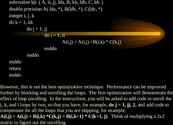
subroutine kji ( A, ii, jj, lda, B, kk, ldb, C, ldc ) double precision A( lda, *), B(ldb, *), C(ldc, *) integer i, j, k do k 1, kk do j 1, jj do i 1, ii A(i,j) A(i,j) B(i,k) * C(k,j) enddo enddo enddo return enddo However, this is not the best optimization technique. Performance can be improved further by blocking and unrolling the loops. The first optimization will demonstrate the effect of loop unrolling. In the instructions, you will be asked to add code to unroll the j, k, and i loops by two, so that you have, for example, do j 1, jj, 2, and add code to compensate for all the loops that you are skipping, for example, A(i,j) A(i,j) B(i,k) *C(k,j) B(i,k 1) * C(k 1, j). Think of multiplying a 2x2 matrix to figure out the unrolling.

The second optimization will demonstrate the effect of blocking, so that, as much as possible, the blocks that are being handled can be kept completely in cache memory. Thus each loop is broken up into blocks (ib, beginning of an i block, ie, end of an i block) and the variables travel from the beginning of the block to the end of the block for each i,j,k. Use blocks of size 32 to start with, if you wish you can experiment with the size of the block to obtain the optimal size. The next logical step is to combine these two optimizations into a routine which is both blocked and unrolled and you will be asked to do this. The final example tries to extract the core of the BLAS dgemm matrix-multiply routine. The blocking and unrolling are retained, but the additional trick here is to optimize the innermost loop. Make sure that it only references items in columns and that it does not reference anything that would not be in a column. To that end, B is copied and transposed into the temp matrix T(k,i) B(i,k). Then multiplying B(i,k)*C(k,j) is equivalent to multiplying T(k,i)*C(k,j) (notice the k index occurs only in the row). Also, we do not store the result in A(i,j) A(i,j) B(i,k)*C(k,j) but in a temporary variable T1 T1 T(k,j)*C(k,j). The effect of this is the inner k-loop has no extraneous references. After the inner loop has executed, A(i,j) is set to its correct value.

mydgemm: do kb 1, kk, blk ke min(kb blk-1,kk) do ib 1, ii, blk ie min(ib blk-1, ii) do i ib,ie do k kb, ke T(k-kb 1, i-ib 1) B(i,k) enddo enddo do jb 1, jj, blk je min(jb blk-1, jj) do j jb, je, 2 do i ib, ie, 2 T1 0.0d0 T2 0.0d0 T3 0.0d0 T4 0.0d0 do k kb, ke T1 T1 T (k-kb 1,i-ib 1)*C(k,j) T2 T2 T(k-kb 1, i-ib 2)*C(k,j) T3 T3 T(k-kb 1, i-ib 1)*C(k,j 1) T4 T4 T(k-kb 1, i-ib 2)*C(k,j 1) enddo A(i,j) A(i,j) T1 A(i 1,j) A(i 1, j) T2 A(i,j 1) A(i, j 1) T3 A(i 1, j 1) A(i 1, j 1) T4 enddo enddo enddo enddo

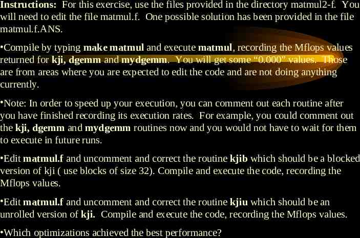
Instructions: For this exercise, use the files provided in the directory matmul2-f. You will need to edit the file matmul.f. One possible solution has been provided in the file matmul.f.ANS. Compile by typing make matmul and execute matmul, recording the Mflops values returned for kji, dgemm and mydgemm. You will get some “0.000” values. Those are from areas where you are expected to edit the code and are not doing anything currently. Note: In order to speed up your execution, you can comment out each routine after you have finished recording its execution rates. For example, you could comment out the kji, dgemm and mydgemm routines now and you would not have to wait for them to execute in future runs. Edit matmul.f and uncomment and correct the routine kjib which should be a blocked version of kji ( use blocks of size 32). Compile and execute the code, recording the Mflops values. Edit matmul.f and uncomment and correct the routine kjiu which should be an unrolled version of kji. Compile and execute the code, recording the Mflops values. Which optimizations achieved the best performance?

Why was this performance achieved? (Review the information about dgemm and mydgemm for the answer) Why is the performance of dgemm worse than that of mydgemm? (mydgemm extracts the core of dgemm to make it somewhat simpler to understand. In doing so it throws away the parts of dgemm which are generic and applicable to any size matrix. Since mydgemm cannot handle arbitrary size matrices it is somewhat faster than dgemm but less useful).