Multicriteria Decision Making Analytical Hierarchy Processes

Multicriteria Decision Making Analytical Hierarchy Processes

Overview of AHP GP answers “how much?”, whereas AHP answers “which one?” AHP developed by Saati Method for ranking decision alternatives and selecting the best one when the decision maker has multiple objectives, or criteria

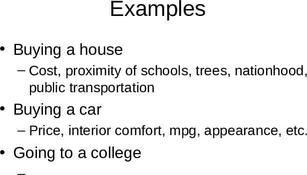
Examples Buying a house – Cost, proximity of schools, trees, nationhood, public transportation Buying a car – Price, interior comfort, mpg, appearance, etc. Going to a college –

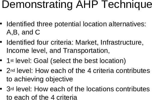
Demonstrating AHP Technique Identified three potential location alternatives: A,B, and C Identified four criteria: Market, Infrastructure, Income level, and Transportation, 1st level: Goal (select the best location) 2nd level: How each of the 4 criteria contributes to achieving objective 3rd level: How each of the locations contributes to each of the 4 criteria

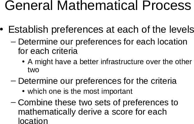
General Mathematical Process Establish preferences at each of the levels – Determine our preferences for each location for each criteria A might have a better infrastructure over the other two – Determine our preferences for the criteria which one is the most important – Combine these two sets of preferences to mathematically derive a score for each location

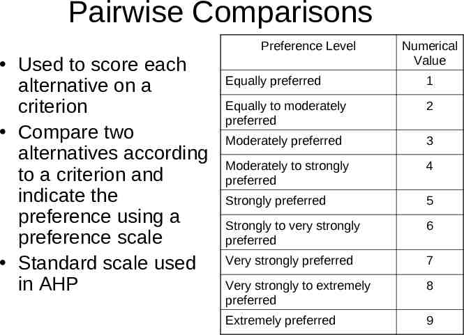
Pairwise Comparisons Used to score each alternative on a criterion Compare two alternatives according to a criterion and indicate the preference using a preference scale Standard scale used in AHP Preference Level Numerical Value Equally preferred 1 Equally to moderately preferred 2 Moderately preferred 3 Moderately to strongly preferred 4 Strongly preferred 5 Strongly to very strongly preferred 6 Very strongly preferred 7 Very strongly to extremely preferred 8 Extremely preferred 9

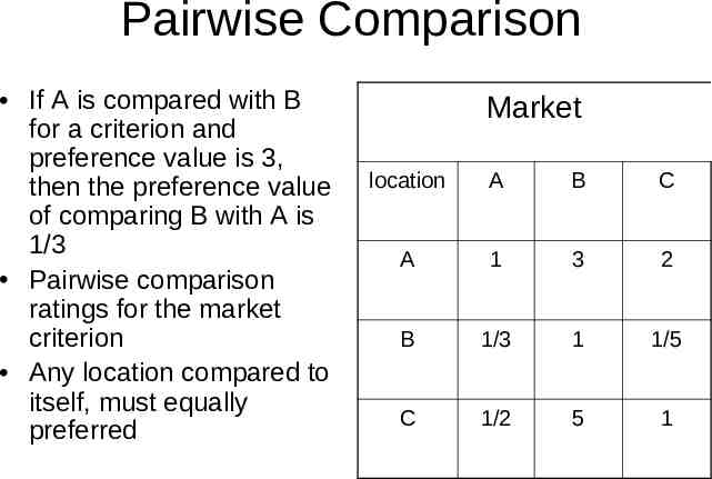
Pairwise Comparison If A is compared with B for a criterion and preference value is 3, then the preference value of comparing B with A is 1/3 Pairwise comparison ratings for the market criterion Any location compared to itself, must equally preferred Market location A B C A 1 3 2 B 1/3 1 1/5 C 1/2 5 1

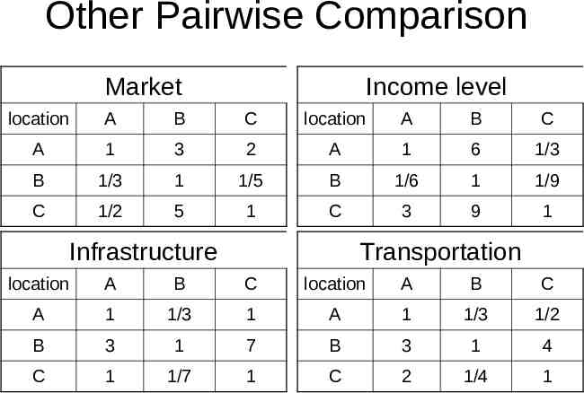
Other Pairwise Comparison Market Income level location A B C location A B C A 1 3 2 A 1 6 1/3 B 1/3 1 1/5 B 1/6 1 1/9 C 1/2 5 1 C 3 9 1 Infrastructure Transportation location A B C location A B C A 1 1/3 1 A 1 1/3 1/2 B 3 1 7 B 3 1 4 C 1 1/7 1 C 2 1/4 1

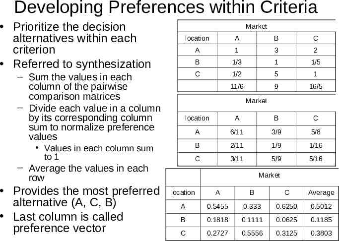
Developing Preferences within Criteria Prioritize the decision alternatives within each criterion Referred to synthesization Market – Sum the values in each column of the pairwise comparison matrices – Divide each value in a column by its corresponding column sum to normalize preference values location A B C A 1 3 2 B 1/3 1 1/5 C 1/2 5 1 11/6 9 16/5 Market location A B C A 6/11 3/9 5/8 B 2/11 1/9 1/16 C 3/11 5/9 5/16 Values in each column sum to 1 – Average the values in each row Provides the most preferred alternative (A, C, B) Last column is called preference vector Market location A B C Average A 0.5455 0.333 0.6250 0.5012 B 0.1818 0.1111 0.0625 0.1185 C 0.2727 0.5556 0.3125 0.3803

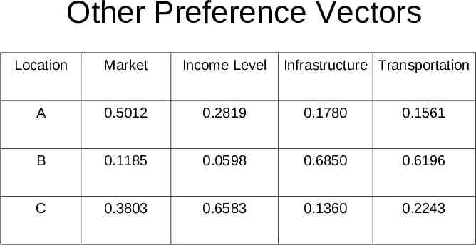
Other Preference Vectors Location Market Income Level Infrastructure Transportation A 0.5012 0.2819 0.1780 0.1561 B 0.1185 0.0598 0.6850 0.6196 C 0.3803 0.6583 0.1360 0.2243

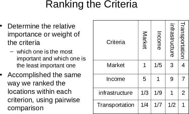
Ranking the Criteria infrastructure Transportation Accomplished the same way we ranked the locations within each criterion, using pairwise comparison Income – which one is the most important and which one is the least important one Criteria Market Determine the relative importance or weight of the criteria Market 1 1/5 3 4 Income 5 1 9 7 1 2 infrastructure Transportation 1/3 1/9 1/4 1/7 1/2 1

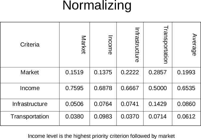
Normalizing 0.1375 0.2222 0.2857 0.1993 Income 0.7595 0.6878 0.6667 0.5000 0.6535 Infrastructure 0.0506 0.0764 0.0741 0.1429 0.0860 Transportation 0.0380 0.0983 0.0370 0.0714 0.0612 Income level is the highest priority criterion followed by market Average Infrastructure Transportation Income 0.1519 Market Market Criteria

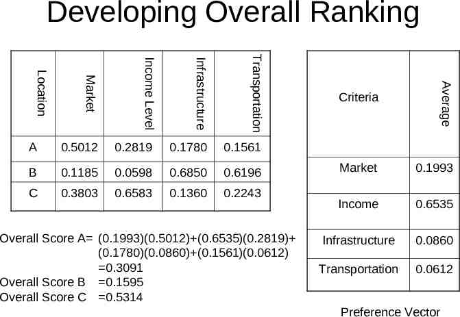
Developing Overall Ranking Transportation 0.1561 B 0.1185 0.0598 0.6850 0.6196 C 0.3803 0.6583 0.1360 0.2243 Overall Score A (0.1993)(0.5012) (0.6535)(0.2819) (0.1780)(0.0860) (0.1561)(0.0612) 0.3091 Overall Score B 0.1595 Overall Score C 0.5314 Average Infrastructure 0.1780 Income Level 0.2819 Market 0.5012 Location A Criteria Market 0.1993 Income 0.6535 Infrastructure 0.0860 Transportation 0.0612 Preference Vector

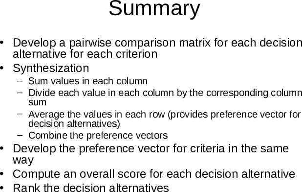
Summary Develop a pairwise comparison matrix for each decision alternative for each criterion Synthesization – Sum values in each column – Divide each value in each column by the corresponding column sum – Average the values in each row (provides preference vector for decision alternatives) – Combine the preference vectors Develop the preference vector for criteria in the same way Compute an overall score for each decision alternative Rank the decision alternatives

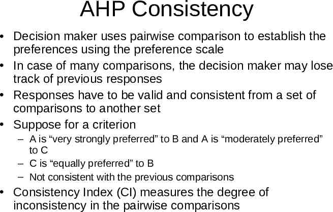
AHP Consistency Decision maker uses pairwise comparison to establish the preferences using the preference scale In case of many comparisons, the decision maker may lose track of previous responses Responses have to be valid and consistent from a set of comparisons to another set Suppose for a criterion – A is “very strongly preferred” to B and A is “moderately preferred” to C – C is “equally preferred” to B – Not consistent with the previous comparisons Consistency Index (CI) measures the degree of inconsistency in the pairwise comparisons

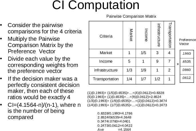
CI Computation Pairwise Comparison Matrix infrastructure Transportation Market 1 1/5 3 4 Income 5 1 9 7 infrastructure 1/3 1/9 1 2 .0860 Transportation 1/4 1/7 1/2 1 .0612 Income Criteria Market Consider the pairwise comparisons for the 4 criteria Multiply the Pairwise Comparison Matrix by the Preference Vector Divide each value by the corresponding weights from the preference vector If the decision maker was a perfectly consistent decision maker, then each of these ratios would be exactly 4 CI (4.1564-n)/(n-1), where n is the number of being compared (1)(0.1993) (1/5)(0.6535) (4)(0.0612) 0.8328 (5)(0.1993) (1)(0.6535) (9)(0.0612) 2.8524 (1/3)(0.1993) (1/9)(0.6535) (2)(0.0612) 0.3474 (1/4)(0.1993) (1/7)(0.6535) (1)(0.0612) 0.2473 0.8328/0.1993 4.1786 2.8524/06535 4.3648 0.3474/.0760 4.0401 0.2473/0.0612 4.0422 Ave 4.1564 Preference Vector .1993 * .6535

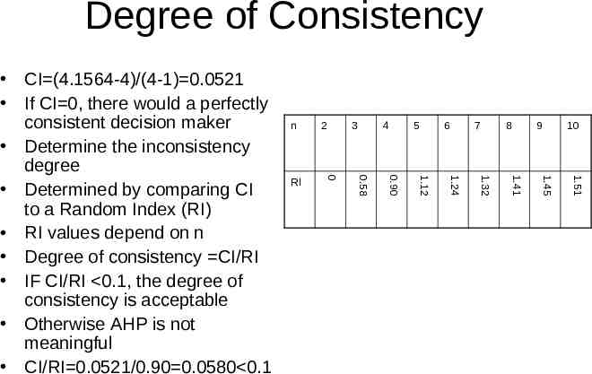
Degree of Consistency n 3 4 5 6 7 8 9 10 1.51 1.45 1.41 1.32 1.24 1.12 0.90 0.58 RI 2 0 CI (4.1564-4)/(4-1) 0.0521 If CI 0, there would a perfectly consistent decision maker Determine the inconsistency degree Determined by comparing CI to a Random Index (RI) RI values depend on n Degree of consistency CI/RI IF CI/RI 0.1, the degree of consistency is acceptable Otherwise AHP is not meaningful CI/RI 0.0521/0.90 0.0580 0.1

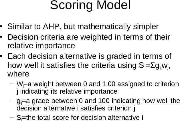
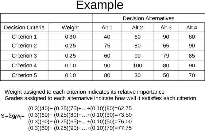
Scoring Model Similar to AHP, but mathematically simpler Decision criteria are weighted in terms of their relative importance Each decision alternative is graded in terms of how well it satisfies the criteria using Si Σgijwj, where – Wj a weight between 0 and 1.00 assigned to criterion j indicating its relative importance – gij a grade between 0 and 100 indicating how well the decision alternative i satisfies criterion j – Si the total score for decision alternative i

Example Decision Alternatives Decision Criteria Weight Alt.1 Alt.2 Alt.3 Alt.4 Criterion 1 0.30 40 60 90 60 Criterion 2 0.25 75 80 65 90 Criterion 3 0.25 60 90 79 85 Criterion 4 0.10 90 100 80 90 Criterion 5 0.10 80 30 50 70 Weight assigned to each criterion indicates its relative importance Grades assigned to each alternative indicate how well it satisfies each criterion (0.3)(40) (0.25)(75) (0.10)(80) 62.75 Si Σgijwj (0.3)(60) (0.25)(80) (0.10)(30) 73.50 (0.3)(90) (0.25)(65) (0.10)(50) 76.00 (0.3)(60) (0.25)(90) (0.10)(70) 77.75

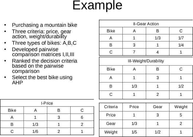
Example II-Gear Action Purchasing a mountain bike Three criteria: price, gear action, weight/durability Three types of bikes: A,B,C Developed pairwise comparison matrices I,II,III Ranked the decision criteria based on the pairwise comparison Select the best bike using AHP Bike A B C A 1 1/3 1/7 B 3 1 1/4 C 7 4 1 III-Weight/Durability I-Price Bike A B C A 1 3 1 B 1/3 1 1/2 C 1 2 1 Criteria Price Gear Weight Price 1 3 5 Bike A B C A 1 3 6 B 1/3 1 2 Gear 1/3 1 2 C 1/6 2 1 Weight 1/5 1/2 1