@Micki Hill 10.09.2021 UK Stata Conference 2021 Introducing stipw:

@Micki Hill 10.09.2021 UK Stata Conference 2021 Introducing stipw: inverse probability weighted parametric survival models Micki Hill1 PC Lambert1,2 and MJ Crowther2 University of Leicester; Leicester (UK), 2Karolinska Institutet; Stockholm (Sweden) 1 stipw (logit tvar tmvarlist [, tmoptions]) [if] [in] , d(distname) [options]

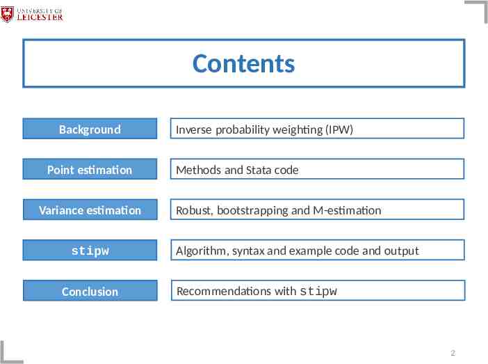
Contents Background Point estimation Variance estimation stipw Conclusion Inverse probability weighting (IPW) Methods and Stata code Robust, bootstrapping and M-estimation Algorithm, syntax and example code and output Recommendations with stipw 2

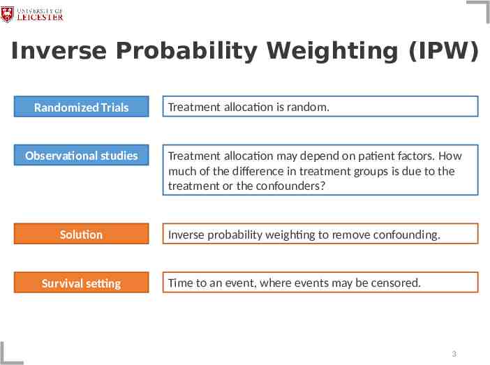
Inverse Probability Weighting (IPW) Randomized Trials Observational studies Solution Survival setting Treatment allocation is random. Treatment allocation may depend on patient factors. How much of the difference in treatment groups is due to the treatment or the confounders? Inverse probability weighting to remove confounding. Time to an event, where events may be censored. 3

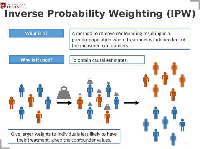
Inverse Probability Weighting (IPW) What is it? Why is it used? A method to remove confounding resulting in a pseudo-population where treatment is independent of the measured confounders. To obtain causal estimates. Give larger weights to individuals less likely to have their treatment, given the confounder values. 4

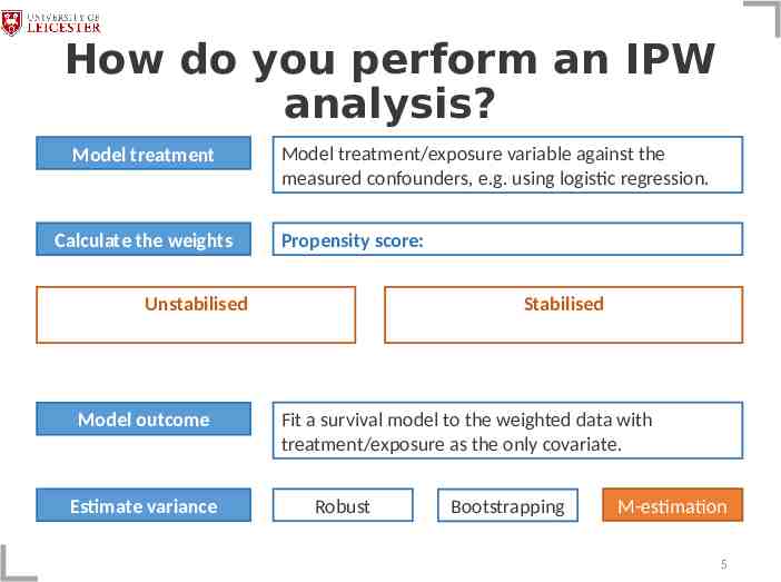
How do you perform an IPW analysis? Model treatment Calculate the weights Model treatment/exposure variable against the measured confounders, e.g. using logistic regression. Propensity score: Unstabilised Model outcome Estimate variance Stabilised Fit a survival model to the weighted data with treatment/exposure as the only covariate. Robust Bootstrapping M-estimation 5

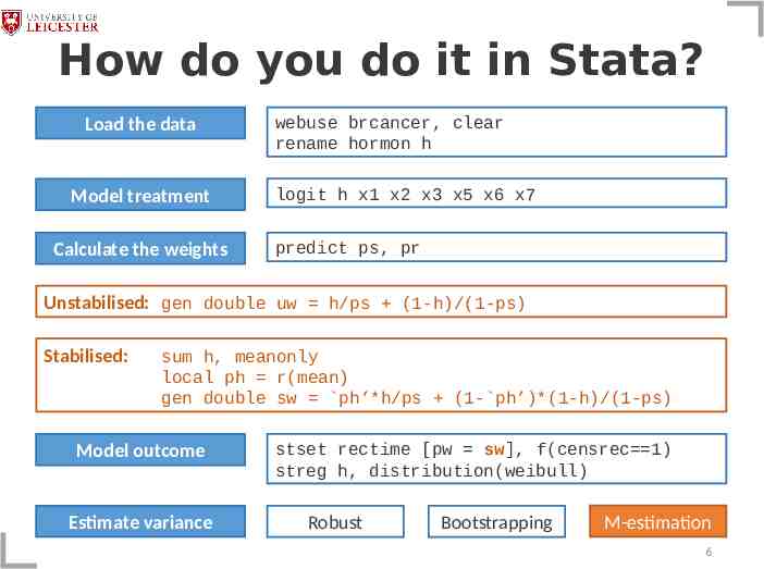
How do you do it in Stata? Load the data Model treatment Calculate the weights webuse brcancer, clear rename hormon h logit h x1 x2 x3 x5 x6 x7 predict ps, pr Unstabilised: gen double uw h/ps (1-h)/(1-ps) Stabilised: sum h, meanonly local ph r(mean) gen double sw ph’*h/ps (1- ph’)*(1-h)/(1-ps) Model outcome Estimate variance stset rectime [pw sw], f(censrec 1) streg h, distribution(weibull) Robust Bootstrapping M-estimation 6

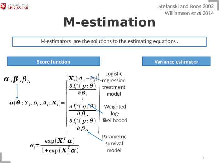
M-estimation Stefanski and Boos 2002 Williamson et al 2014 M-estimators are the solutions to the estimating equations . Score function Logistic 𝑿 𝑖 ( 𝐴 𝑖 𝑒 𝑖 ) regression 𝑙𝑤 𝑖 ( 𝑦 ; 𝜃) treatment 𝛽1 model 𝜶 , 𝜷 , 𝛽𝐴 𝒖 ( 𝜽 ; 𝑌 𝑖 , 𝛿𝑖 , 𝐴 𝑖 , 𝑿 𝑖 ) 𝑒 𝑖 Variance estimator ( ) 𝑙 ( 𝑦 ; 𝜃) 𝛽𝑝 𝑙𝑤 𝑖 ( 𝑦 ; 𝜃) 𝛽𝐴 𝑤 𝑖 exp( 𝑿 𝑇𝑖 𝜶) 𝑇 1 exp ( 𝑿 𝑖 𝜶 ) Weighted loglikelihoood Parametric survival model 7

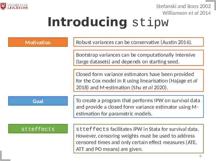
Stefanski and Boos 2002 Williamson et al 2014 Introducing stipw Motivation Robust variances can be conservative (Austin 2016). Bootstrap variances can be computationally intensive (large datasets) and depends on starting seed. Closed form variance estimators have been provided for the Cox model in R using linearisation (Hajage et al 2018) and M-estimation (Shu et al 2020). Goal To create a program that performs IPW on survival data and provide a closed form variance estimator using Mestimation for parametric models. stteffects stteffects facilitates IPW in Stata for survival data. However, censoring weights must be used to address censored times and only certain effect measures (ATE, ATT and PO means) are given. 8

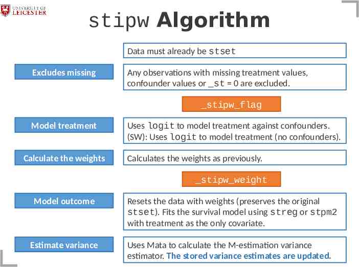
stipw Algorithm Data must already be stset Excludes missing Any observations with missing treatment values, confounder values or st 0 are excluded. stipw flag Model treatment Calculate the weights Uses logit to model treatment against confounders. (SW): Uses logit to model treatment (no confounders). Calculates the weights as previously. stipw weight Model outcome Resets the data with weights (preserves the original stset). Fits the survival model using streg or stpm2 with treatment as the only covariate. Estimate variance Uses Mata to calculate the M-estimation variance estimator. The stored variance estimates are updated.9

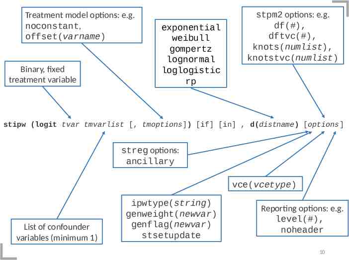
Treatment model options: e.g. noconstant, offset(varname) Binary, fixed treatment variable exponential weibull gompertz lognormal loglogistic rp stpm2 options: e.g. df(#), dftvc(#), knots(numlist), knotstvc(numlist) stipw (logit tvar tmvarlist [, tmoptions]) [if] [in] , d(distname) [options] streg options: ancillary vce(vcetype) List of confounder variables (minimum 1) ipwtype(string) genweight(newvar) genflag(newvar) stsetupdate Reporting options: e.g. level(#), noheader 10

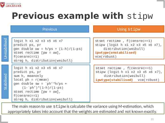
Previous example with stipw Stabilised Unstabilised Previous Using stipw logit h x1 x2 x3 x5 x6 x7 predict ps, pr gen double uw h/ps (1-h)/(1-ps) stset rectime [pw uw], f(censrec 1) streg h, distribution(weibull) stset rectime , f(censrec 1) stipw (logit h x1 x2 x3 x5 x6 x7), distribution(weibull) ipwtype(unstabilised) vce(robust) logit h x1 x2 x3 x5 x6 x7 predict ps, pr sum h, meanonly local ph r(mean) gen double sw ph’*h/ps (1- ph’)*(1-h)/(1-ps) stset rectime [pw uw], f(censrec 1) streg h, distribution(weibull) stset rectime , f(censrec 1) stipw (logit h x1 x2 x3 x5 x6 x7), distribution(weibull) ipwtype(stabilised) vce(robust) The main reason to use stipw is calculate the variance using M-estimation, which appropriately takes into account that the weights are estimated and not known exactly. 11

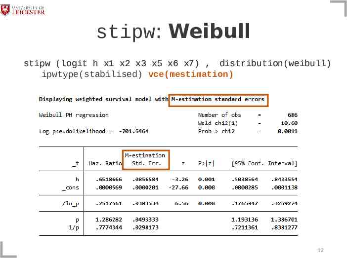
stipw: Weibull stipw (logit h x1 x2 x3 x5 x6 x7) , distribution(weibull) ipwtype(stabilised) vce(mestimation) 12

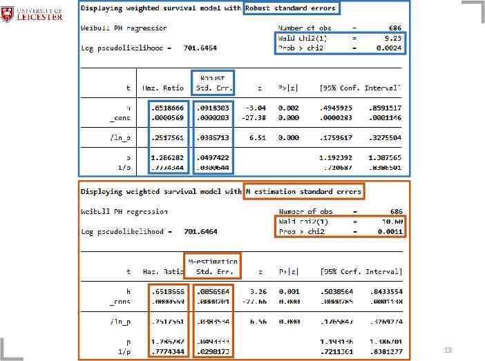
13

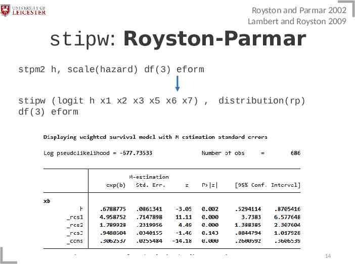
Royston and Parmar 2002 Lambert and Royston 2009 stipw: Royston-Parmar stpm2 h, scale(hazard) df(3) eform stipw (logit h x1 x2 x3 x5 x6 x7) , distribution(rp) df(3) eform 14

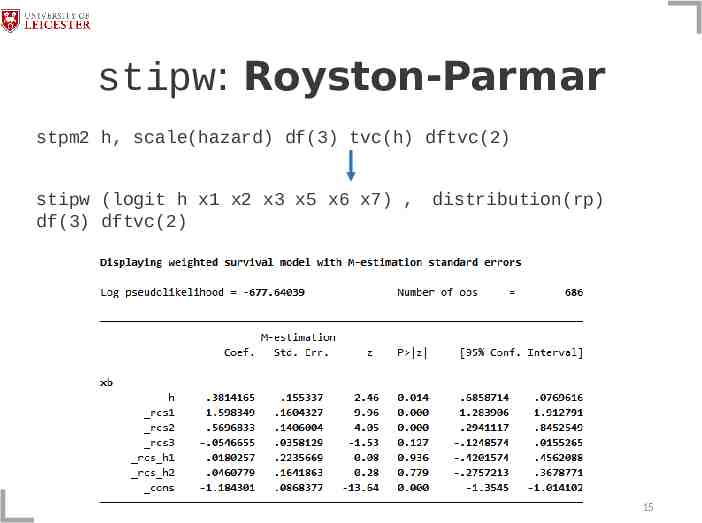
stipw: Royston-Parmar stpm2 h, scale(hazard) df(3) tvc(h) dftvc(2) stipw (logit h x1 x2 x3 x5 x6 x7) , distribution(rp) df(3) dftvc(2) 15

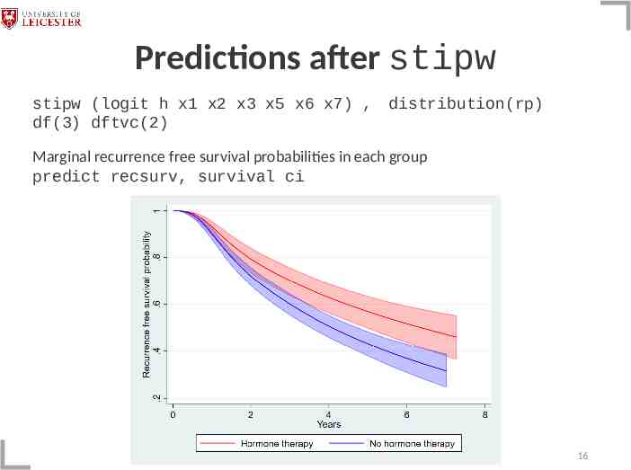
Predictions after stipw stipw (logit h x1 x2 x3 x5 x6 x7) , distribution(rp) df(3) dftvc(2) Marginal recurrence free survival probabilities in each group predict recsurv, survival ci 16

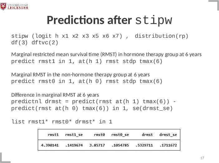
Predictions after stipw stipw (logit h x1 x2 x3 x5 x6 x7) , distribution(rp) df(3) dftvc(2) Marginal restricted mean survival time (RMST) in hormone therapy group at 6 years predict rmst1 in 1, at(h 1) rmst stdp tmax(6) Marginal RMST in the non-hormone therapy group at 6 years predict rmst0 in 1, at(h 0) rmst stdp tmax(6) Difference in marginal RMST at 6 years predictnl drmst predict(rmst at(h 1) tmax(6)) predict(rmst at(h 0) tmax(6)) in 1, se(drmst se) list rmst1* rmst0* drmst* in 1 17

Conclusion The stipw package facilitates IPW with survival data and allows the user to calculate robust or M-estimation standard errors. M-estimation appropriately takes into account that weights are estimated. The variance of a wide range of causal effects can be estimated using the M-estimation variance estimator. This is done using standard postestimation commands, as the stored variance estimates are updated. We recommend stipw for large datasets, where treatment prevalence is common and when bootstrapping may be too computationally intensive. Extensions to stipw could include different treatment models (e.g. probit), adding the Cox model, different types of weights (Mao et al 2018), clustered data, competing risks and more. @Micki Hill [email protected] 18

References Austin PC. Variance estimation when using inverse probability of treatment weighting (IPTW) with survival analysis. Statistics in Medicine. 2016;35(30):5642-55. Hajage D, Chauvet G, Belin L, Lafourcade A, Tubach F, De Rycke Y. Closed‐form variance estimator for weighted propensity score estimators with survival outcome. Biometrical Journal. 2018;60(6):1151-63. Lambert PC, Royston P. Further development of flexible parametric models for survival analysis. The Stata Journal. 2009;9(2):265-90. Mao H, Li L, Yang W, Shen Y. On the propensity score weighting analysis with survival outcome: Estimands, estimation, and inference. Statistics in medicine. 2018;37(26):3745-63. Royston P, Parmar MKB. Flexible parametric proportional‐hazards and proportional ‐odds models for censored survival data, with application to prognostic modelling and estimation of treatment effects. Statistics in Medicine. 2002;21(15):2175-97. Shu D, Young JG, Toh S, Wang R. Variance estimation in inverse probability weighted Cox models. Biometrics. 2020. Stefanski LA, Boos DD. The calculus of M-estimation. The American Statistician. 2002;56(1):29-38. Williamson EJ, Forbes A, White IR. Variance reduction in randomised trials by inverse probability weighting using the propensity score. Statistics in Medicine. 2014;33(5):721-37. 19