Management Science 461 Lecture 4b – P-median problems September

Management Science 461 Lecture 4b – P-median problems September 30, 2008

Problem with coverage Coverage models are best for “worst case problems” We want to ensure good response for even the most remote demand node in the network Density does not drive the model, the lack of density does Central assumption: if it’s close, it’s covered 2

Problem with coverage Coverage model treats each demand node the same (max coverage the exception) A more appropriate measure is needed to find good average solutions This is what median problems are good for 3

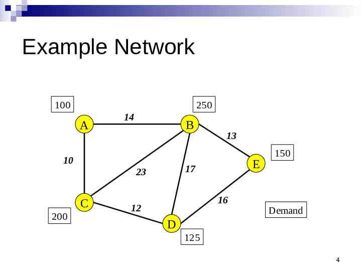
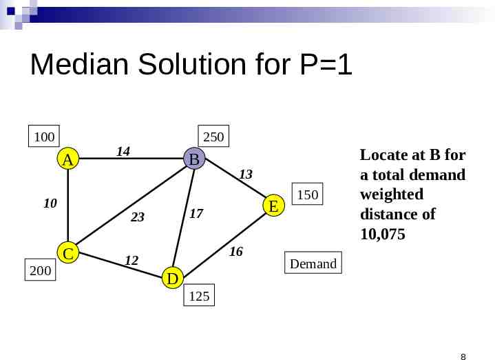
Example Network 100 250 A 14 B 10 200 E 17 23 C 13 16 12 150 Demand D 125 4

Problem Description Need to locate facilities and allocate customers to the facility so as to minimize total distance traveled Decision variables Locate at j or not: binary value Xj Allocate customer i to facility j: binary Yij 5

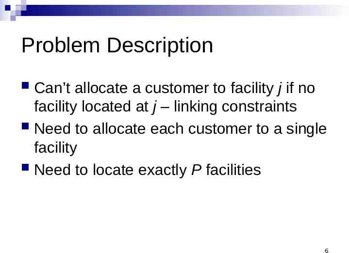
Problem Description Can’t allocate a customer to facility j if no facility located at j – linking constraints Need to allocate each customer to a single facility Need to locate exactly P facilities 6

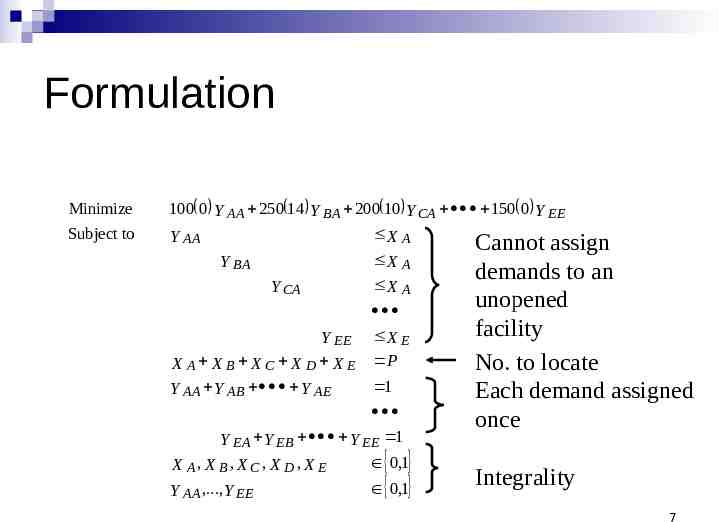
Formulation Minimize 100 0 Y AA 250 14 Y BA 200 10 Y CA 150 0 Y EE Subject to Y AA X A Y BA X A Y CA Y EE X A X B XC X D X E Y AA Y AB Y AE X A X E P 1 Y EA Y EB Y EE 1 X A, X B , X C , X D , X E Y AA ,.,Y EE 0,1 0,1 Cannot assign demands to an unopened facility No. to locate Each demand assigned once Integrality 7

Median Solution for P 1 100 A 10 14 B 13 E 17 23 C 200 250 16 12 D 150 Locate at B for a total demand weighted distance of 10,075 Demand 125 8

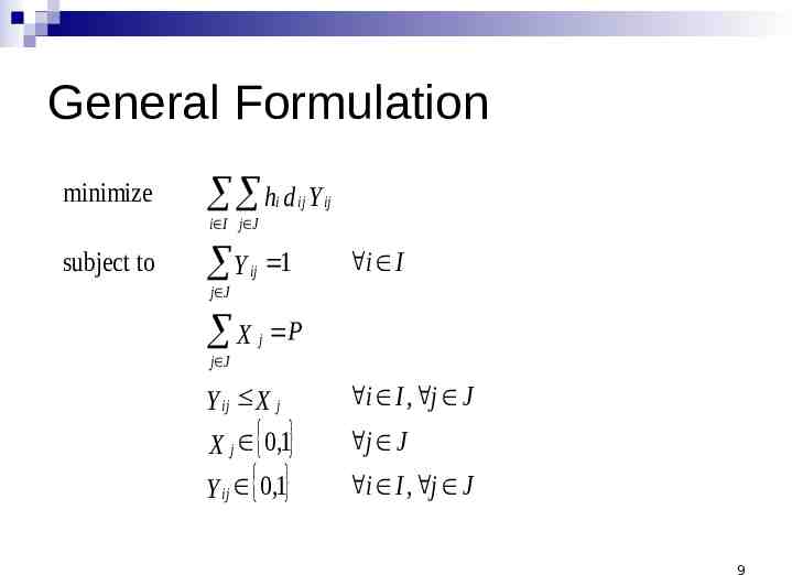
General Formulation minimize h d i ij Y ij i I j J subject to Y 1 ij i I j J X j P j J Y ij X j X j 0,1 i I , j J Y ij 0,1 i I , j J j J 9

Extensions Facility costs Need to convert total travel to a cost to incorporate both in the same model Relax “one customer, one facility” Add a capacity constraint on facilities All these things make the problem harder than it already is 10

Solving 1-Median Locating a single facility is straightforward: Gravity model if location unrestricted and/or no network defined Enumeration of all candidate sites Demo in Excel 11

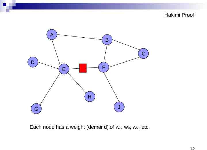
Hakimi Proof A B C D F E H G J Each node has a weight (demand) of wA, wB, wC, etc. 12

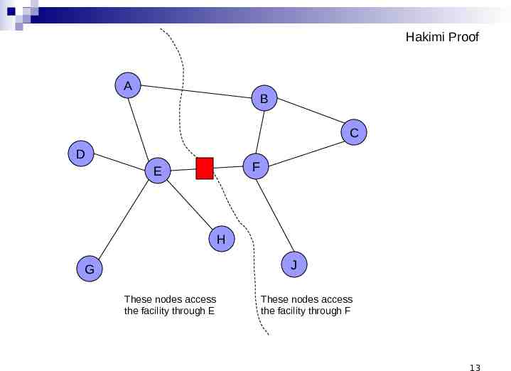
Hakimi Proof A B C D F E H J G These nodes access the facility through E These nodes access the facility through F 13

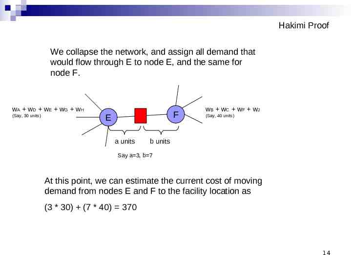
Hakimi Proof We collapse the network, and assign all demand that would flow through E to node E, and the same for node F. wA wD wE wG wH (Say, 30 units) F E a units wB wC wF wJ (Say, 40 units) b units Say a 3, b 7 At this point, we can estimate the current cost of moving demand from nodes E and F to the facility location as (3 * 30) (7 * 40) 370 14

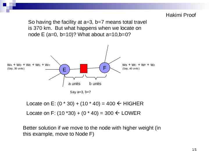
Hakimi Proof So having the facility at a 3, b 7 means total travel is 370 km. But what happens when we locate on node E (a 0, b 10)? What about a 10,b 0? wA wD wE wG wH (Say, 30 units) F E a units wB wC wF wJ (Say, 40 units) b units Say a 3, b 7 Locate on E: (0 * 30) (10 * 40) 400 HIGHER Locate on F: (10 *30) (0 * 40) 300 LOWER Better solution if we move to the node with higher weight (in this example, move to Node F) 15

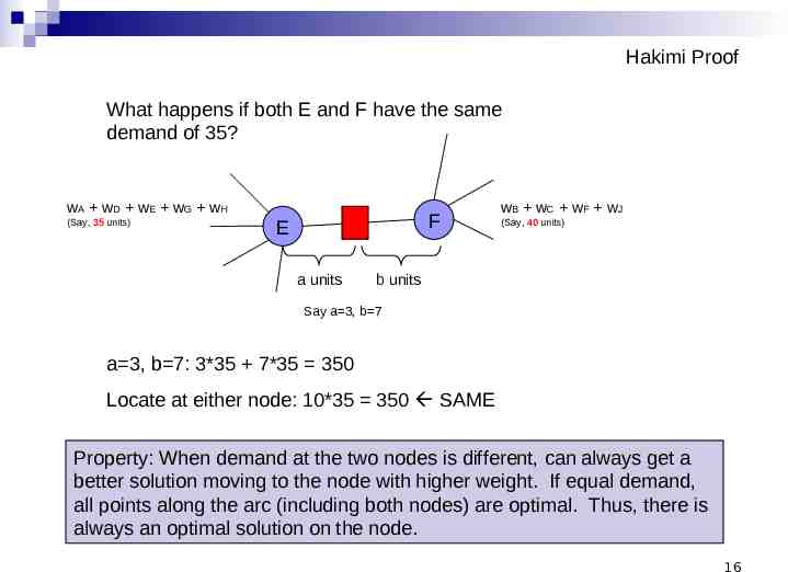
Hakimi Proof What happens if both E and F have the same demand of 35? wA wD wE wG wH (Say, 35 units) F E a units wB wC wF wJ (Say, 40 units) b units Say a 3, b 7 a 3, b 7: 3*35 7*35 350 Locate at either node: 10*35 350 SAME Property: When demand at the two nodes is different, can always get a better solution moving to the node with higher weight. If equal demand, all points along the arc (including both nodes) are optimal. Thus, there is always an optimal solution on the node. 16

Complexity of P-median Original problem has n choose p solutions: n! / [(n-p)!p!] For n 10 and p 3, 120 solutions For n 100 and p 15, 2.5E17 solutions At 1,000,000,000 solutions per second, how long would total enumeration take? “non-polynomial” problem; heuristic solutions needed 17

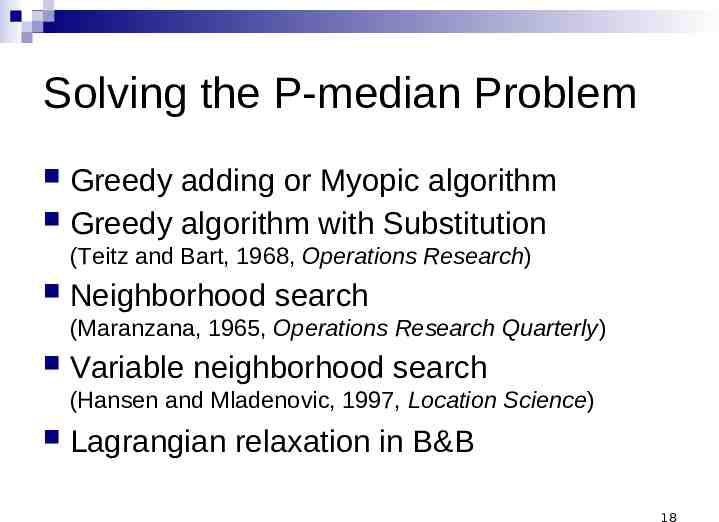
Solving the P-median Problem Greedy adding or Myopic algorithm Greedy algorithm with Substitution (Teitz and Bart, 1968, Operations Research) Neighborhood search (Maranzana, 1965, Operations Research Quarterly) Variable neighborhood search (Hansen and Mladenovic, 1997, Location Science) Lagrangian relaxation in B&B 18

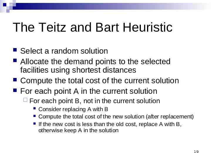
The Teitz and Bart Heuristic Select a random solution Allocate the demand points to the selected facilities using shortest distances Compute the total cost of the current solution For each point A in the current solution For each point B, not in the current solution Consider replacing A with B Compute the total cost of the new solution (after replacement) If the new cost is less than the old cost, replace A with B, otherwise keep A in the solution 19

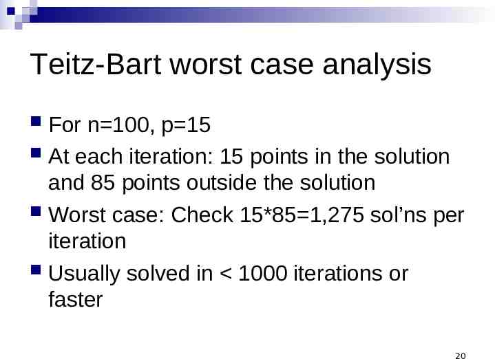
Teitz-Bart worst case analysis For n 100, p 15 At each iteration: 15 points in the solution and 85 points outside the solution Worst case: Check 15*85 1,275 sol’ns per iteration Usually solved in 1000 iterations or faster 20