Making statistic claims Corpus Linguistics Richard

Making statistic claims Corpus Linguistics Richard Xiao [email protected]

Update on assignments Deadline for submission (email submission): Friday 31 May 2013 The Harvard referencing style Assignment A – Corpus study: introduction; synopsis / overview, critical review of data, method of analysis, conclusion etc; conclusions, bibliography Corpus Linguistics Conferences 2001-2011: http://ucrel.lancs.ac.uk/cl2013/past-confs.php UCCTS2008: http://www.lancs.ac.uk/fass/projects/corpus/UCCTS2008Proceedings/ UCCTS2010: http://www.lancs.ac.uk/fass/projects/corpus/UCCTS2010Proceedings/ – Corpus tool: Introduction; description of the tool, its main features and functions; your critical evaluation of the tool: how well it does the jobs it is supposed to do; user interface, powerfulness, etc; conclusions; bibliography Assignment B – Introduction; literature review; methodology; results and discussions; conclusions; bibliography Option B: A 3,500-word essay, similar to Assignment B

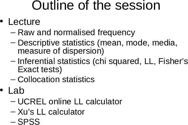
Outline of the session Lecture – Raw and normalised frequency – Descriptive statistics (mean, mode, media, measure of dispersion) – Inferential statistics (chi squared, LL, Fisher’s Exact tests) – Collocation statistics Lab – UCREL online LL calculator – Xu’s LL calculator – SPSS

Quantitative analysis Corpus analysis is both qualitative and quantitative One of the advantages of corpora is that they can readily provide quantitative data which intuitions cannot provide reliably “The use of quantification in corpus linguistics typically goes well beyond simple counting” (McEnery and Wilson 2001: 81) – What can we do with those numbers and counts derived from a corpus?

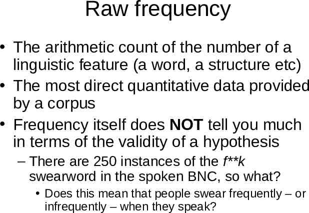
Raw frequency The arithmetic count of the number of a linguistic feature (a word, a structure etc) The most direct quantitative data provided by a corpus Frequency itself does NOT tell you much in terms of the validity of a hypothesis – There are 250 instances of the f**k swearword in the spoken BNC, so what? Does this mean that people swear frequently – or infrequently – when they speak?

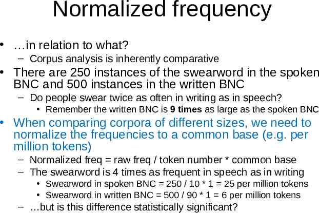
Normalized frequency in relation to what? – Corpus analysis is inherently comparative There are 250 instances of the swearword in the spoken BNC and 500 instances in the written BNC – Do people swear twice as often in writing as in speech? Remember the written BNC is 9 times as large as the spoken BNC When comparing corpora of different sizes, we need to normalize the frequencies to a common base (e.g. per million tokens) – Normalized freq raw freq / token number * common base – The swearword is 4 times as frequent in speech as in writing Swearword in spoken BNC 250 / 10 * 1 25 per million tokens Swearword in written BNC 500 / 90 * 1 6 per million tokens – but is this difference statistically significant?

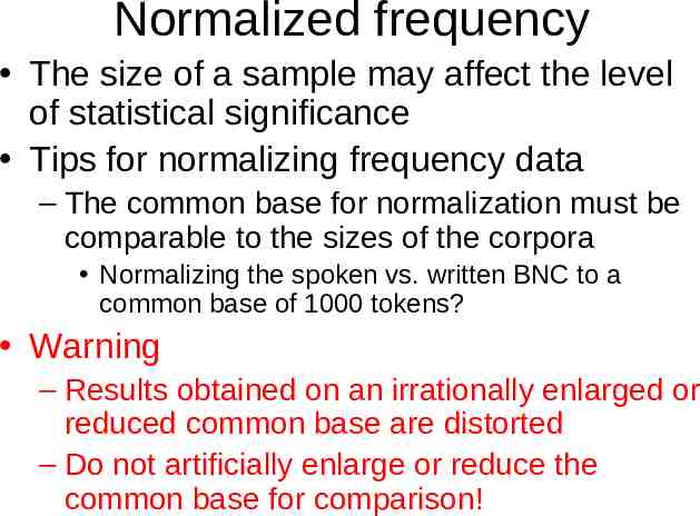
Normalized frequency The size of a sample may affect the level of statistical significance Tips for normalizing frequency data – The common base for normalization must be comparable to the sizes of the corpora Normalizing the spoken vs. written BNC to a common base of 1000 tokens? Warning – Results obtained on an irrationally enlarged or reduced common base are distorted – Do not artificially enlarge or reduce the common base for comparison!

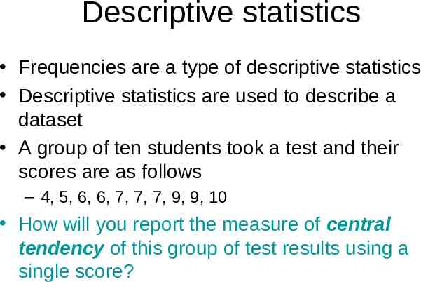
Descriptive statistics Frequencies are a type of descriptive statistics Descriptive statistics are used to describe a dataset A group of ten students took a test and their scores are as follows – 4, 5, 6, 6, 7, 7, 7, 9, 9, 10 How will you report the measure of central tendency of this group of test results using a single score?

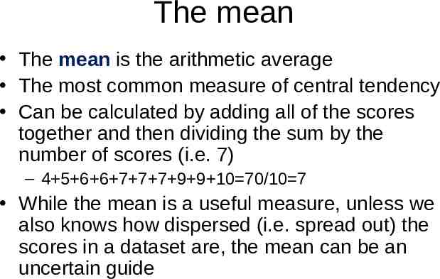
The mean The mean is the arithmetic average The most common measure of central tendency Can be calculated by adding all of the scores together and then dividing the sum by the number of scores (i.e. 7) – 4 5 6 6 7 7 7 9 9 10 70/10 7 While the mean is a useful measure, unless we also knows how dispersed (i.e. spread out) the scores in a dataset are, the mean can be an uncertain guide

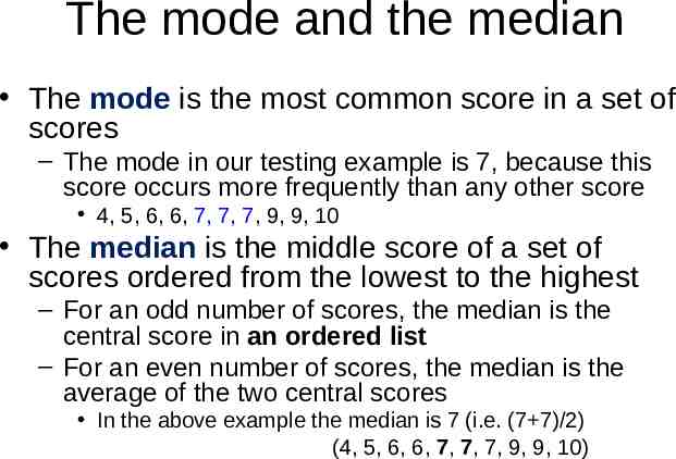
The mode and the median The mode is the most common score in a set of scores – The mode in our testing example is 7, because this score occurs more frequently than any other score 4, 5, 6, 6, 7, 7, 7, 9, 9, 10 The median is the middle score of a set of scores ordered from the lowest to the highest – For an odd number of scores, the median is the central score in an ordered list – For an even number of scores, the median is the average of the two central scores In the above example the median is 7 (i.e. (7 7)/2) (4, 5, 6, 6, 7, 7, 7, 9, 9, 10)

Measure of dispersion: range The range is a simple way to measure the dispersion of a set of data – The difference between the highest and lowest frequencies / scores – In our testing example the range is 6 (i.e. highest 10 – lowest 4) Only a poor measure of dispersion – An unusually high or low score in a dataset may make the range unreasonably large, thus giving a distorted picture of the dataset

Measure of dispersion: variance The variance measures the distance of each score in the dataset from the mean – In our test results, the variance of the score 4 is 3 (i.e. 7–4); and the variance of the score 9 is 2 (9–7) For the whole dataset, the sum of these differences is always zero – Some scores will be above the mean while some will be below the mean Meaningless to use variance to measure the dispersion of a whole dataset

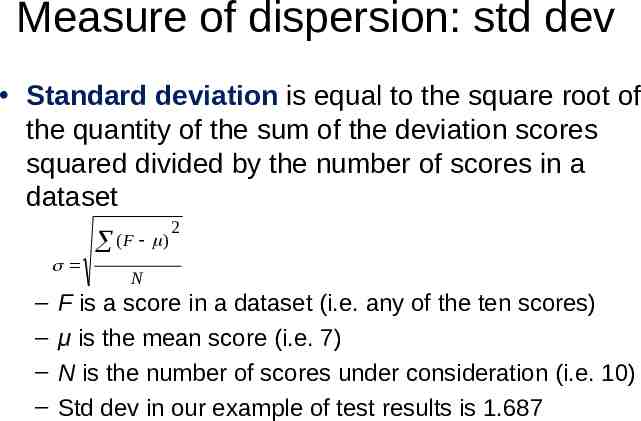
Measure of dispersion: std dev Standard deviation is equal to the square root of the quantity of the sum of the deviation scores squared divided by the number of scores in a dataset (F ) – – – – 2 N F is a score in a dataset (i.e. any of the ten scores) μ is the mean score (i.e. 7) N is the number of scores under consideration (i.e. 10) Std dev in our example of test results is 1.687

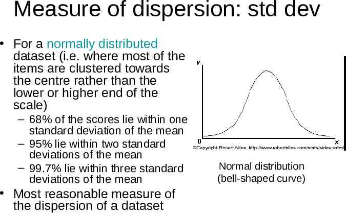
Measure of dispersion: std dev For a normally distributed dataset (i.e. where most of the items are clustered towards the centre rather than the lower or higher end of the scale) – 68% of the scores lie within one standard deviation of the mean – 95% lie within two standard deviations of the mean – 99.7% lie within three standard deviations of the mean Most reasonable measure of the dispersion of a dataset Normal distribution (bell-shaped curve)

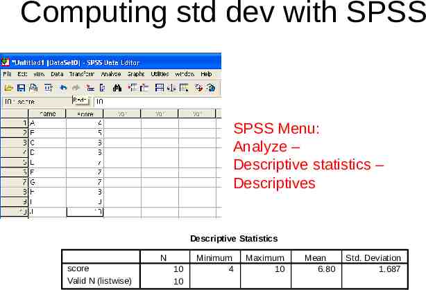
Computing std dev with SPSS SPSS Menu: Analyze – Descriptive statistics – Descriptives Descriptive Statistics N score Valid N (listwise) 10 10 Minimum 4 Maximum 10 Mean 6.80 Std. Deviation 1.687

Inferential statistics Descriptive statistics are useful in summarizing a dataset Inferential statistics are typically used to formulate or test a hypothesis – Using statistical measures to test whether or not any differences observed are statistically significant Tests of statistical significance – chi-square test – log-likelihood (LL) test – Fisher’s Exact test Collocation statistics – Mutual information (MI) – z score

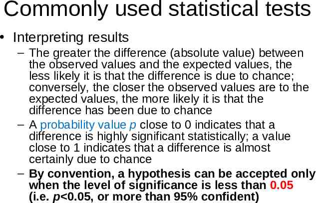
Statistical significance In testing a linguistic hypothesis, it would be nice to be 100% sure that the hypothesis can be accepted However, one can never be 100% sure in real life cases – There is always the possibility that the differences observed between two corpora or samples have been due to chance In our swearword example, it is 4 times as frequent in speech as in writing We need to use a statistical test to help us to decide whether this difference is statistically significant The level of statistical significance the level of our confidence in accepting a given hypothesis – The closer the likelihood is to 100%, the more confident we can be One must be more than 95% confident that the observed differences have not arisen by chance

Commonly used statistical tests Chi square test – compares the difference between the observed values (e.g. the actual frequencies extracted from corpora) and the expected values (e.g. the frequencies that one would expect if no factor other than chance was affecting the frequencies) Log likelihood test (LL) – Similar, but more reliable as LL does not assume that data is normally distributed – The preferred test for statistic significance

Commonly used statistical tests Interpreting results – The greater the difference (absolute value) between the observed values and the expected values, the less likely it is that the difference is due to chance; conversely, the closer the observed values are to the expected values, the more likely it is that the difference has been due to chance – A probability value p close to 0 indicates that a difference is highly significant statistically; a value close to 1 indicates that a difference is almost certainly due to chance – By convention, a hypothesis can be accepted only when the level of significance is less than 0.05 (i.e. p 0.05, or more than 95% confident)

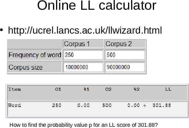
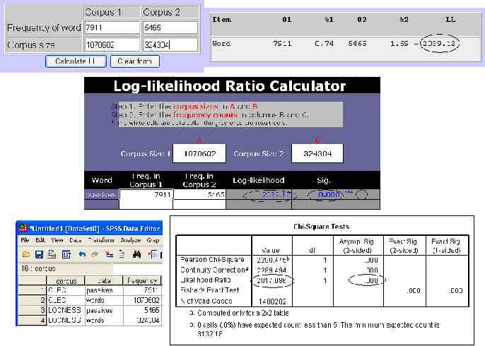
Online LL calculator http://ucrel.lancs.ac.uk/llwizard.html How to find the probability value p for an LL score of 301.88?

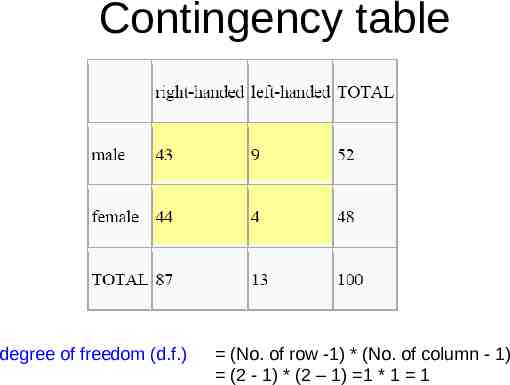
Contingency table degree of freedom (d.f.) (No. of row -1) * (No. of column - 1) (2 - 1) * (2 – 1) 1 * 1 1

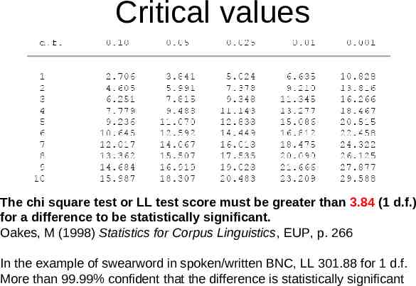
Critical values The chi square test or LL test score must be greater than 3.84 (1 d.f.) for a difference to be statistically significant. Oakes, M (1998) Statistics for Corpus Linguistics, EUP, p. 266 In the example of swearword in spoken/written BNC, LL 301.88 for 1 d.f. More than 99.99% confident that the difference is statistically significant

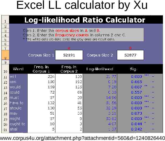
Excel LL calculator by Xu www.corpus4u.org/attachment.php?attachmentid 560&d 1240826440

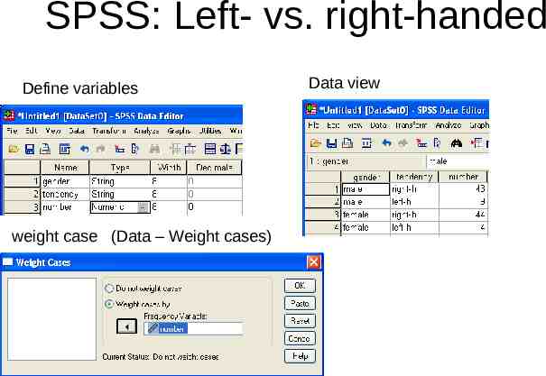
SPSS: Left- vs. right-handed Define variables weight case (Data – Weight cases) Data view

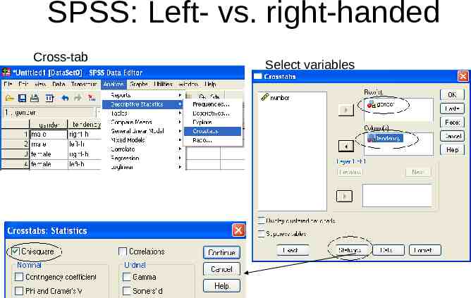
SPSS: Left- vs. right-handed Cross-tab Select variables

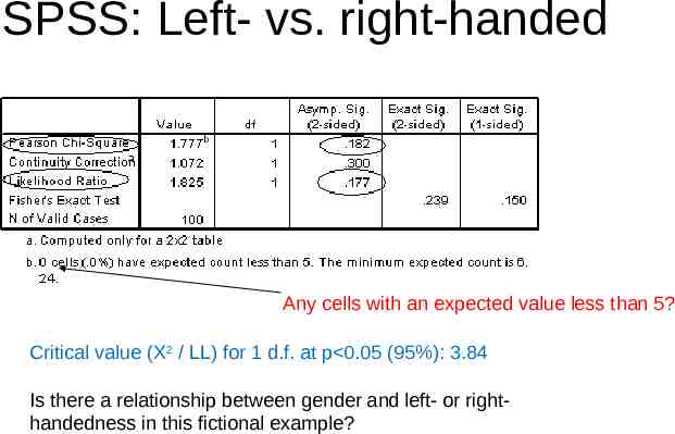
SPSS: Left- vs. right-handed Any cells with an expected value less than 5? Critical value (X2 / LL) for 1 d.f. at p 0.05 (95%): 3.84 Is there a relationship between gender and left- or righthandedness in this fictional example?

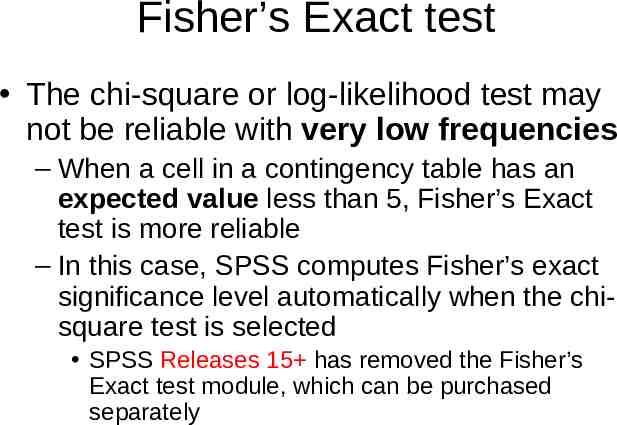
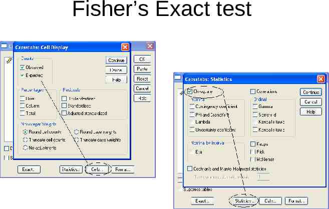
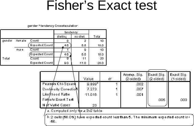
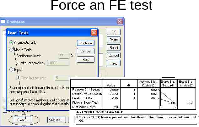
Fisher’s Exact test The chi-square or log-likelihood test may not be reliable with very low frequencies – When a cell in a contingency table has an expected value less than 5, Fisher’s Exact test is more reliable – In this case, SPSS computes Fisher’s exact significance level automatically when the chisquare test is selected SPSS Releases 15 has removed the Fisher’s Exact test module, which can be purchased separately

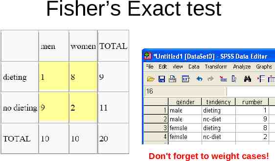
Fisher’s Exact test Don't forget to weight cases!

Fisher’s Exact test

Fisher’s Exact test

Force an FE test

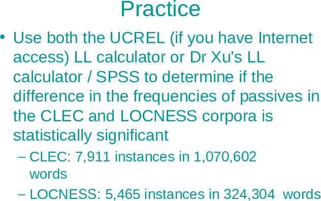
Practice Use both the UCREL (if you have Internet access) LL calculator or Dr Xu’s LL calculator / SPSS to determine if the difference in the frequencies of passives in the CLEC and LOCNESS corpora is statistically significant – CLEC: 7,911 instances in 1,070,602 words – LOCNESS: 5,465 instances in 324,304 words

Collocation statistics Collocation: the habitual or characteristic co-occurrence patterns of words – Can be identified using a statistical approach in CL, e.g. Mutual Information (MI), t test, z score – Can be computed using tools like SPSS or corpus tools like Wordsmith, AntConc, Xaira – Only a brief introduction here More discussions of collocation statistics to be followed

Mutual information Computed by dividing the observed frequency of the co-occurring word in the defined span for the search string (socalled node word), e.g. a 4:4 window, by the expected frequency of the co-occurring word in that span and then taking the logarithm to the base 2 ( 自然对数 ) of the result

Mutual information A measure of collocational strength The higher the MI score, the stronger the link between two items – MI score of 3.0 or higher to be taken as evidence that two items are collocates The closer to 0 the MI score gets, the more likely it is that the two items co-occur by chance A negative MI score indicates that the two items tend to shun each other

The t test Computed by subtracting the expected frequency from the observed frequency and then dividing the result by the standard deviation A t score of 2 or higher is normally considered to be statistically significant The specific probability level can be looked up in a table of t distribution

The z score The z score is the number of standard deviations from the mean frequency The z test compares the observed frequency with the frequency expected if only chance is affecting the distribution A higher z score indicates a greater degree of collocability of an item with the node word A comparison of the effects of these collocation statistics to follow