Lecture 1 Introduction & Basics of Economics Dr. Rajeev Dhawan

Lecture 1 Introduction & Basics of Economics Dr. Rajeev Dhawan Director Given to the EMBA 8400 Class March 19, 2010

Course Objective & Teaching Philosophy Practical Course to Comprehend the Economic Environment so that Managers can make their Decisions Philosophy is that Micro Sectors Add Up to a Macro Environment Optimal Blend of Economics and Real World Experience/Common Sense Train You to Critically Evaluate and Interpret Business Press Writings

Course Layout Week 1 – Basic Economic Concepts and Microeconomics I Week 2 – Microeconomics II and Basics Macroeconomics I Week 3 – Macroeconomics II

Grading Policy TWO RULES: – No Early or Makeup Exams – All Exams are Open Book 20% Quiz #1 (30 minutes) 30% Quiz #2 (45 minutes) 50% Final Comprehensive Exam (2 hours)

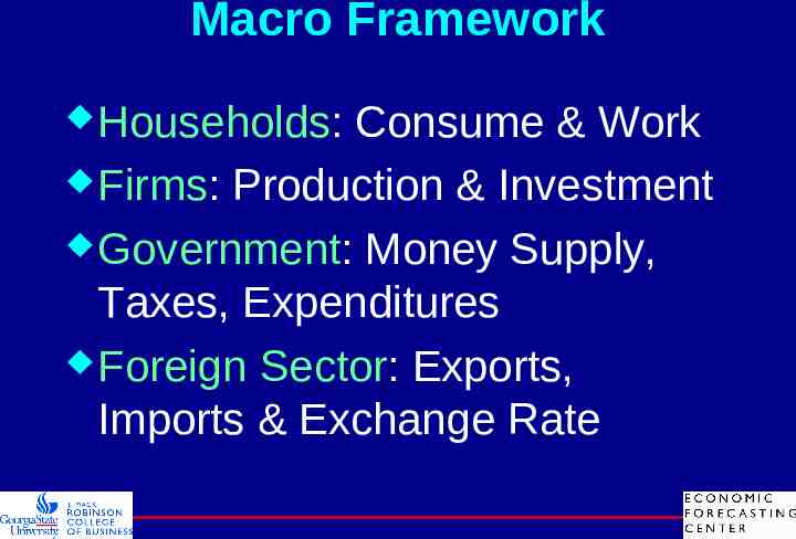
Macro Framework Households: Consume & Work Firms: Production & Investment Government: Money Supply, Taxes, Expenditures Foreign Sector: Exports, Imports & Exchange Rate

Introduction The 10 Principles of Economics

What is Economics? Economics is the study of how we use our scarce productive resources for consumption, now or in future. – Paul Samuelson Resources are scarce: – Society has limited resources and therefore cannot produce all the goods and services people wish to have – Example: clean air & water – Scarcity is not poverty

Basic Questions What to produce in what quantity? How to produce them? When and where to produce? For whom? Who makes economic decisions and by what process?

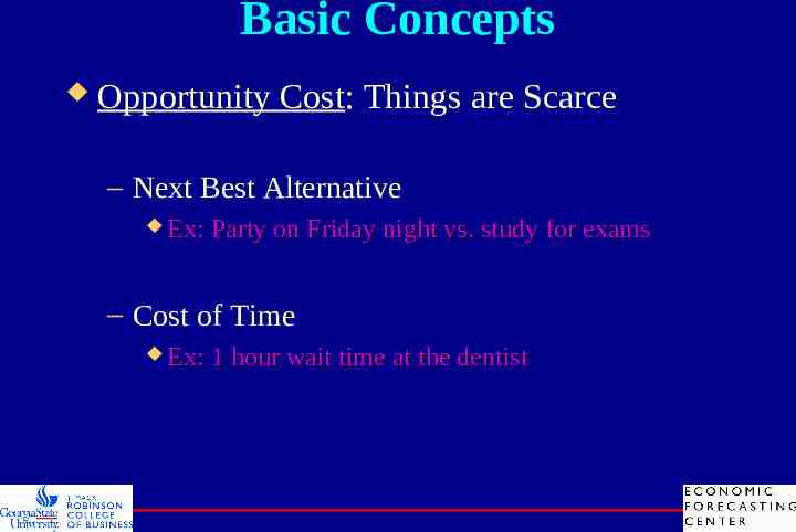
Basic Concepts Opportunity Cost: Things are Scarce – Next Best Alternative Ex: Party on Friday night vs. study for exams – Cost of Time Ex: 1 hour wait time at the dentist

Basic Concepts Marginal Concept: At the Margin Shots of Wild Turk ey Marginal Shot Satisfaction Satisfaction 1 50 20 2 70 10 3 80 5 4 85 1 5 86 0 6 86 Utility: Level of Satisfaction (here, drunkenness)

Basic Concepts Sunk/Fixed Costs: Expenditures Made that Cannot be Recovered – Example: You bought a computer laptop for 1500 A newer, upgraded model costs 1200 The dealer will accept a trade in 400 What do you do?

Winnick’s Voyage to the Bottom of the Sea WSJ; by Andy Kessler First Mover, FCC regulated fixed costs Regulated utility Price protection You can’t lose Traffic / use was of low economic value or cashless Global Crossing couldn't cut prices without running the risk of either failing to cover its debt or being unable to raise more capital Accounting Tricks .

10 Principles of Economics 1. People face tradeoffs : “No such thing as free lunch” Give up one thing to get another – Opportunity Cost (OC) 2. Everything has an OC – whatever must be given up to get that item 3. People make decisions at the margins – increments matter 4. People respond to incentives – e.g. cigarette laws, communism 5. Free Trade is good (for everybody)

10 Principles of Economics 6. Markets organize economic activity - Adam Smith “Invisible Hand” 7. Governments can sometimes improve market outcome 8. A country’s standard of living depends upon its production power (productivity) 9. Prices rise when government prints too much money 10. Phillips curve – short run tradeoff between inflation and unemployment

Branches of Economics Micro: The Study of One Entity (firm, business, people) Macro: The Study of a Collection of Things (national, aggregate)

How are Theories Developed? Decision-Makers – Firms, governments Markets – Place where exchange takes place

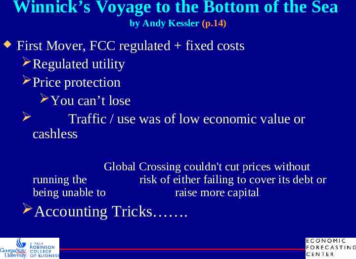
Winnick’s Voyage to the Bottom of the Sea by Andy Kessler (p.14) First Mover, FCC regulated fixed costs Regulated utility Price protection You can’t lose Traffic / use was of low economic value or cashless Global Crossing couldn't cut prices without running the risk of either failing to cover its debt or being unable to raise more capital Accounting Tricks .

Chapter 2 Production

Production What is production? – The activity by which we convert inputs (labor, land & capital) into goods and services What limits production? – Inputs (resources) – Technology Government interference

Circular Flow Diagram Revenue Goods and services sold MARKETS FOR GOODS AND SERVICES Firms sell Households buy Wages, rent, and profit Goods and services bought HOUSEHOLDS Buy and consume goods and services Own and sell factors of production FIRMS Produce and sell goods and services Hire and use factors of production Factors of production Spending Labor, land, MARKETS and capital FOR FACTORS OF PRODUCTION Households sell Firms buy Income Flow of inputs and outputs Flow of dollars

Production Possibilities Frontier Definition: the amount of goods a firm or society can produce given a fixed amount of land, labor and other inputs.

Production Possibilities Frontier Quantity of Pretzels Produced 4,000 D 3,000 a 2,200 2,100 2,000 C E A B 1,000 0 300 d . 600 700 750 b Production possibilities frontier c 1,000 Quantity of Beer Produced

Production Function I Input Y 0 0 MP Y (Production) F (Inputs) 1.00 1 Production Function 1 12 10 1.00 2 1.00 3 3 4 5 5 6 4 2 0 1.00 4 8 Y 2 Y I 0 2 4 6 8 Input Marginal Product: it is the increase in output that 1.00 arises from an additional unit of input. Marginal Product (MP) Output / Input 10

Production Function II Input Y 0 0 Y I2 MP 1.00 1 Production Function 1 120 3.00 4 80 5.00 3 9 16 25 40 0 0 9.00 5 60 20 7.00 4 Y 2 100 2 4 6 8 Input Marginal Product (MP) Output / Input 10

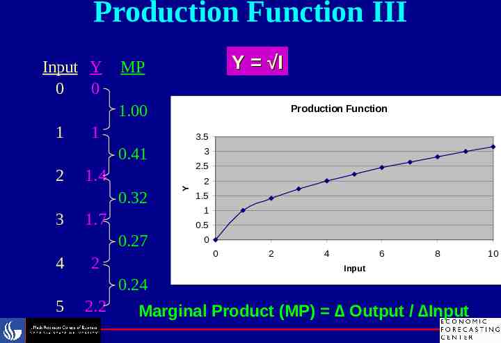
Production Function III Input Y 0 0 Y I MP 1.00 1 Production Function 1 3.5 0.41 1.4 0.32 3 1.7 2 1.5 1 0.5 0.27 4 2.5 Y 2 3 2 0 0 2 4 6 8 Input 0.24 5 2.2 Marginal Product (MP) Output / Input 10

Returns to Scale Returns to Scale: the property of the production function that when you double your inputs, your output either doubles, more than doubles, or less than doubles. 9 DRS Y F 8 MP IRS MP DRS 7 6 CRS Y F 5 4 Y F2 3 2 IRS 1 0 0 1 2 3 4 5 6 7 8 9 10

Chapter 4 Demand & Supply

Some Basic Definitions Market: a group of buyers and sellers of a particular good or service – E.g. Warren Buffet has been buying up junk bonds – E.g. Bars, parties – informal market Stock market – organized market

Example of Supply & Demand Hong Kong chicken flu scare? Price of chicken Mad cow disease in US? Price of beef Oprah bad mouths beef? Price of beef – Amarillo farmers sue her. SARS? (Macro issue )

Demand Quantity demanded (Q): the amount of a good that buyers are willing and able to purchase at a given price (P). QD 0 1 3 6 11 19 10.00 8.00 Price Pints of Beer P 10.00 7.00 5.00 4.00 2.00 0.00 Demand for Beer 6.00 4.00 2.00 0.00 0 5 10 15 Quantity (Pints) 20

Graph Results Demand curve/schedule is downward sloping and shows the relationship between price of a good and the quantity demanded Why downward sloping? – Law of demand: Ceteris Paribus (all other things being equal) the quantity demanded falls when price rises

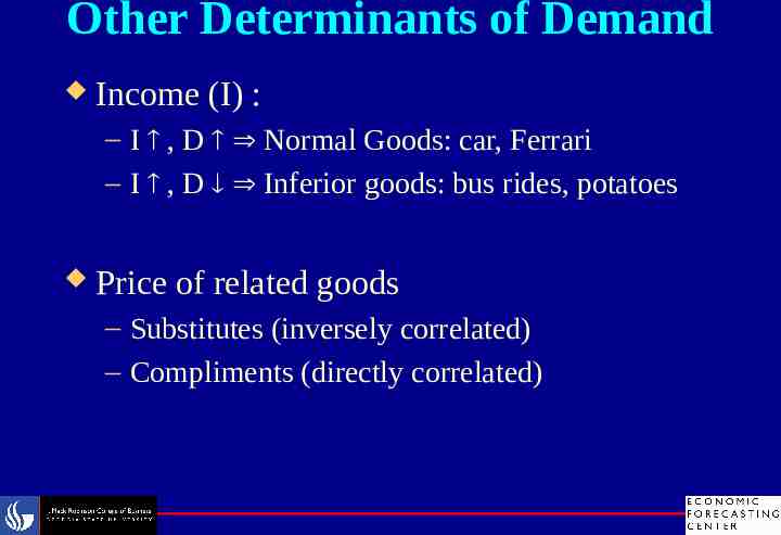
Other Determinants of Demand Income (I) : – I , D Normal Goods: car, Ferrari – I , D Inferior goods: bus rides, potatoes Price of related goods – Substitutes (inversely correlated) – Compliments (directly correlated)

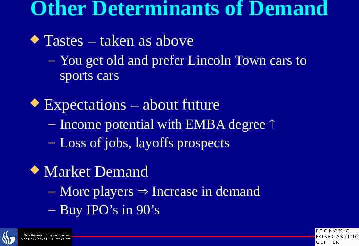
Other Determinants of Demand Tastes – taken as above – You get old and prefer Lincoln Town cars to sports cars Expectations – about future – Income potential with EMBA degree – Loss of jobs, layoffs prospects Market Demand – More players Increase in demand – Buy IPO’s in 90’s

Shifts in Demand Curve Variables that shift the demand curve:

Shifts in the Demand Curve Price of Beer Increase in demand Decrease in demand Demand curve,D3 0 Demand curve, D1 Demand curve, D2 Quantity of Beer

Supply Quantity supplied (Q): the amount of a good that sellers are willing and able to sell at a given price (P). Price Pints of Beer P QS 10.00 12 7.00 7 5.00 4 4.00 3 2.00 1 0.00 0 Supply of Beer - Neighbors 10.00 8.00 6.00 4.00 2.00 0.00 0 2 4 6 8 Quantity (Pints) 10 12

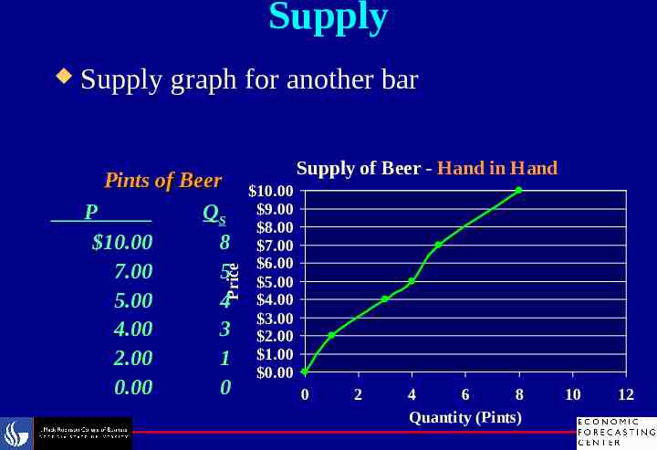
Supply Supply graph for another bar Price Pints of Beer P QS 10.00 8 7.00 5 5.00 4 4.00 3 2.00 1 0.00 0 Supply of Beer - Hand in Hand 10.00 9.00 8.00 7.00 6.00 5.00 4.00 3.00 2.00 1.00 0.00 0 2 4 6 8 Quantity (Pints) 10 12

Determinants of Supply Your own Price Input Prices – Cost of bottle of beer: labor, capital, rent Technology – Smoking laws separation of smoking & drinking Expectations – Future outlook

Shifts in The Supply Curve Variables that shift the supply curve:

Shifts In Supply Curve Price of Beer Supply curve,S3 Decrease in supply Supply curve, S1 Supply curve, S2 Increase in supply 0 Quantity of Beer

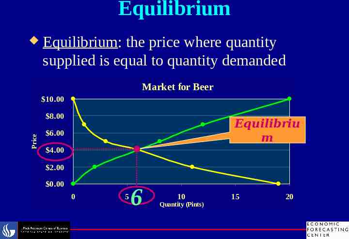
Equilibrium Equilibrium: the price where quantity supplied is equal to quantity demanded Market for Beer 10.00 Price 8.00 Equilibriu m 6.00 4.00 2.00 0.00 0 5 6 10 Quantity (Pints) 15 20

Markets Not In Equilibrium Excess Supply Price of Beer Supply Surplus 6.50 4.00 Demand 0 2 Quantity demanded 6 10 Quantity of Quantity Beer supplied

Markets Not In Equilibrium Excess Demand Price of Beer Supply 4.00 2.50 Shortage Demand 0 2 Quantity supplied 6 10 Quantity demanded Quantity of Beer

Changes in Equilibrium Decide whether the event shifts the supply or demand curve (or both). Decide whether the curve(s) shift(s) to the left or to the right. Use the supply-and-demand diagram to see how the shift affects equilibrium price and quantity.

Changes in Equilibrium An increase in the price of hops reduces the supply of beer An increase in wealth increases demand for beer Price of Beer Price of Beer Suppl y New equilibrium 6.50 S2 S1 New equilibrium 6.50 4.00 Initial equilibrium Initial equilibrium 4.00 D2 Demand D1 0 6 10 Pints of Beer 0 2 6 Pints of Beer

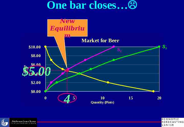
One bar closes New Equilibriu m Market for Beer 10.00 S1 S2 8.00 6.00 Price 5.00 4.00 2.00 0.00 0 4 5 10 Quantity (Pints) 15 20

Chapter 6 Controls on Prices

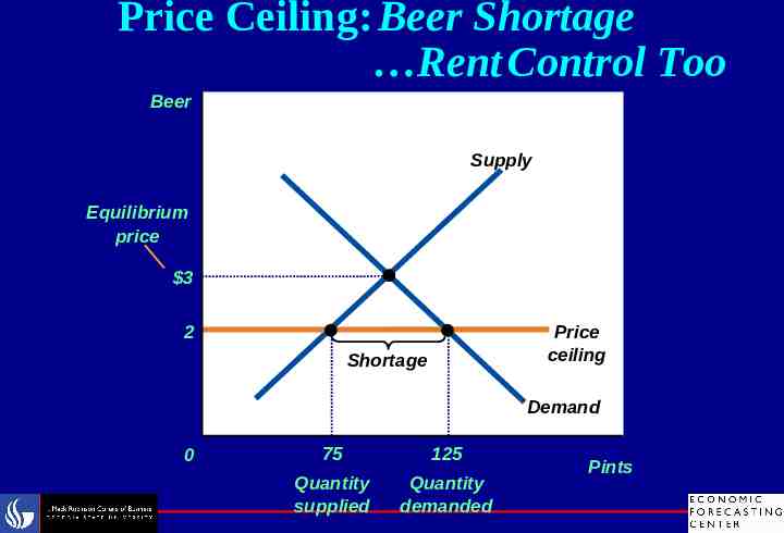
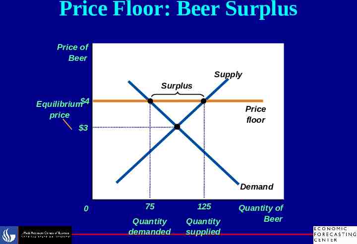
Controls on Prices Price Ceiling (e.g. rent control) – A legal maximum on the price at which a good can be sold. – If the price ceiling is set below the equilibrium price, it leads to a shortage. Price Floor (e.g. minimum wage) – A legal minimum on the price at which a good can be sold. – If the price ceiling is set above the equilibrium price, it leads to a surplus.

Price Ceiling: Beer Shortage Rent Control Too Beer Supply Equilibrium price 3 2 Price ceiling Shortage Demand 0 75 125 Quantity supplied Quantity demanded Pints

Price Floor: Beer Surplus Price of Beer Supply Surplus Equilibrium 4 price Price floor 3 Demand 0 75 125 Quantity demanded Quantity supplied Quantity of Beer