Introduction to R and RStudio Jeff Witmer 9 March 2016

Introduction to R and RStudio Jeff Witmer 9 March 2016

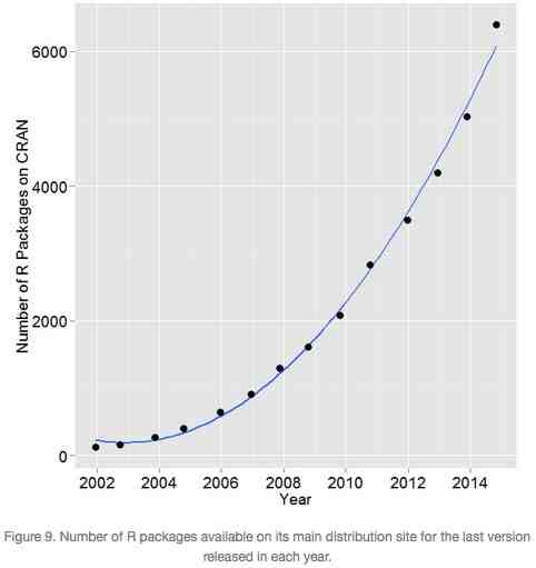
R is A software package for statistical computing and graphics A collection of 6,700 packages (as of June 2015, so more now) A (not ideal) programming language A work environment Widely used Powerful Free

Some history S was developed at Bell Labs, starting in the 1970s R was created in the 1990s by Ross Ihaka and Robert Gentleman R was based on S, with code written in C S largely was used to make good graphs – not an easy thing in 1975. R, like S, is quite good for graphing. For lots of examples, see http://rgraphgallery.blogspot.com/ or http://www.r-graph-gallery.com/ See ggplot2-cheatsheet-2.0.pdf (Or for more detail, see http://docs.ggplot2.org/current/

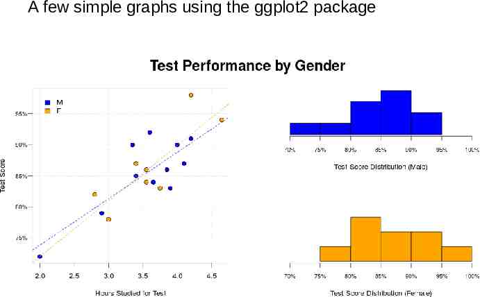
A few simple graphs using the ggplot2 package

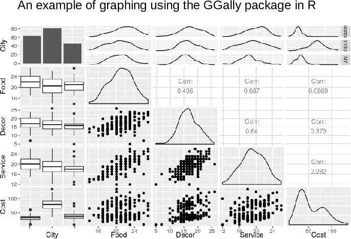
An example of graphing using the GGally package in R

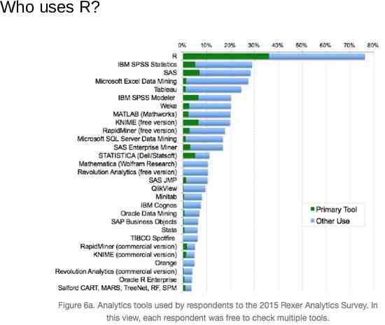
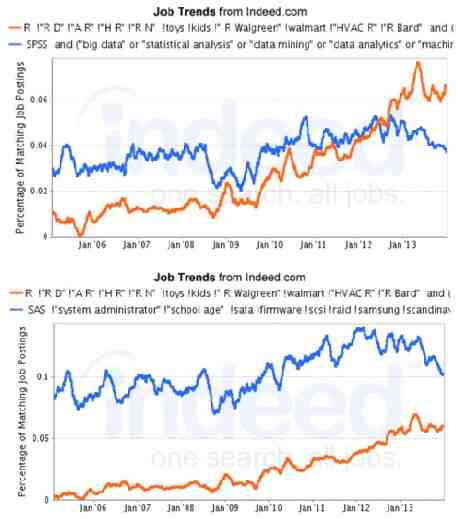
Who uses R?

RStudio is An Integrated Development Environment (IDE) for R A gift, from J.J. Allaire (Macalester College, ‘91) to the world An easy (easier) way to use R Available as a desktop product or, as used at OC, run off of a file server. Free – unless you want the newest version, with more bells and whistles, and you are not eligible for the educational discount ( free) R supports rpubs – see http://rpubs.com/jawitmer

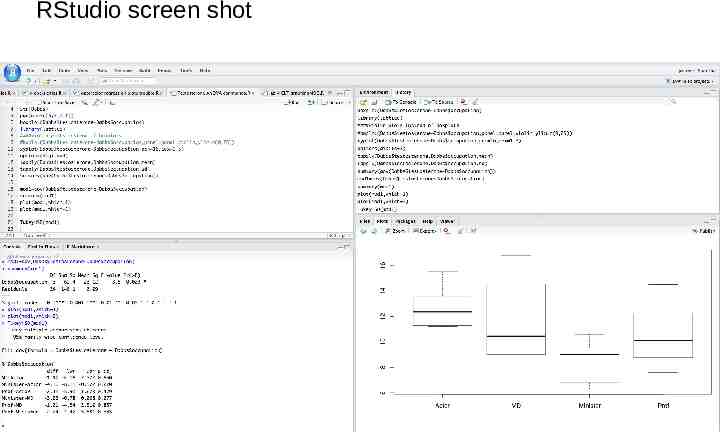
RStudio screen shot

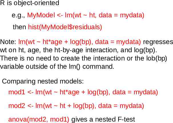
R is object-oriented e.g., MyModel - lm(wt ht, data mydata) then hist(MyModel residuals) Note: lm(wt ht*age log(bp), data mydata) regresses wt on ht, age, the ht-by-age interaction, and log(bp). There is no need to create the interaction or the lob(bp) variable outside of the lm() command. Comparing nested models: mod1 - lm(wt ht*age log(bp), data mydata) mod2 - lm(wt ht log(bp), data mydata) anova(mod2, mod1) gives a nested F-test

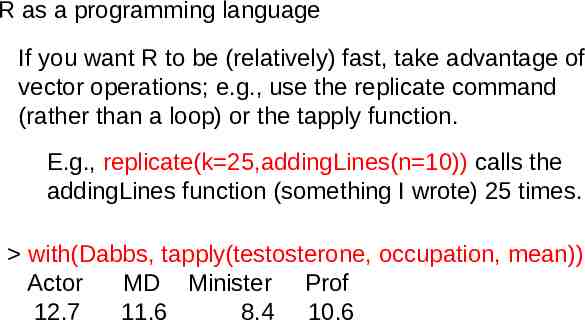
R as a programming language If you want R to be (relatively) fast, take advantage of vector operations; e.g., use the replicate command (rather than a loop) or the tapply function. E.g., replicate(k 25,addingLines(n 10)) calls the addingLines function (something I wrote) 25 times. with(Dabbs, tapply(testosterone, occupation, mean)) Actor MD Minister Prof 12.7 11.6 8.4 10.6

If you want to know how to do something in R See the “Minimal R.pdf” handout Go to the Quick-R.com page (http://www.statmethods.net/) Google “How do I do xxx in R?” A standing joke among R users is that the answer is always “There are many ways to do that in R.” See http://swirlstats.com/ See https://www.datacamp.com/home

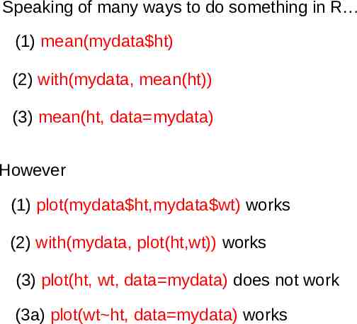
Speaking of many ways to do something in R (1) mean(mydata ht) (2) with(mydata, mean(ht)) (3) mean(ht, data mydata) However (1) plot(mydata ht,mydata wt) works (2) with(mydata, plot(ht,wt)) works (3) plot(ht, wt, data mydata) does not work (3a) plot(wt ht, data mydata) works

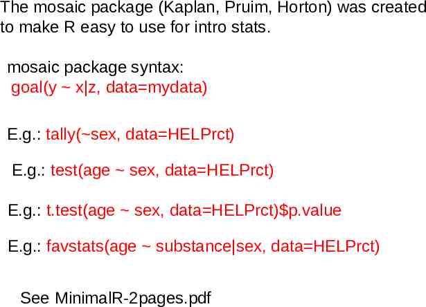
The mosaic package (Kaplan, Pruim, Horton) was created to make R easy to use for intro stats. mosaic package syntax: goal(y x z, data mydata) E.g.: tally( sex, data HELPrct) E.g.: test(age sex, data HELPrct) E.g.: t.test(age sex, data HELPrct) p.value E.g.: favstats(age substance sex, data HELPrct) See MinimalR-2pages.pdf

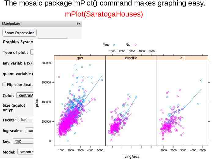
The mosaic package mPlot() command makes graphing easy. mPlot(SaratogaHouses)

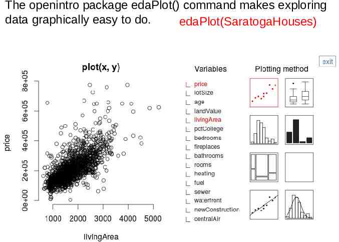
The openintro package edaPlot() command makes exploring data graphically easy to do. edaPlot(SaratogaHouses)

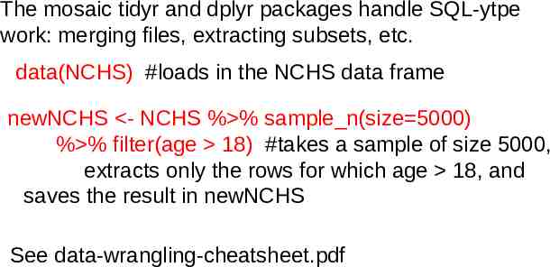
The mosaic tidyr and dplyr packages handle SQL-ytpe work: merging files, extracting subsets, etc. data(NCHS) #loads in the NCHS data frame newNCHS - NCHS % % sample n(size 5000) % % filter(age 18) #takes a sample of size 5000, extracts only the rows for which age 18, and saves the result in newNCHS See data-wrangling-cheatsheet.pdf

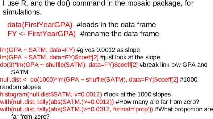
I use R, and the do() command in the mosaic package, for simulations. data(FirstYearGPA) #loads in the data frame FY - FirstYearGPA) #rename the data frame lm(GPA SATM, data FY) #gives 0.0012 as slope lm(GPA SATM, data FY) coeff[2] #just look at the slope do(3)*lm(GPA shuffle(SATM), data FY) coeff[2] #break link b/w GPA and SATM null.dist - do(1000)*lm(GPA shuffle(SATM), data FY) coeff[2] #1000 random slopes histogram(null.dist SATM, v 0.0012) #look at the 1000 slopes with(null.dist, tally(abs(SATM.) 0.0012)) #How many are far from zero? with(null.dist, tally(abs(SATM.) 0.0012, format 'prop')) #What proportion are far from zero?

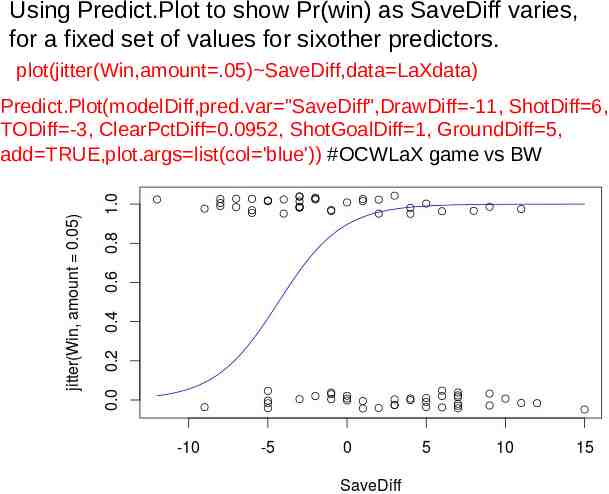
Using Predict.Plot to show Pr(win) as SaveDiff varies, for a fixed set of values for sixother predictors. plot(jitter(Win,amount .05) SaveDiff,data LaXdata) Predict.Plot(modelDiff,pred.var "SaveDiff",DrawDiff -11, ShotDiff 6, TODiff -3, ClearPctDiff 0.0952, ShotGoalDiff 1, GroundDiff 5, add TRUE,plot.args list(col 'blue')) #OCWLaX game vs BW