Hydrologic Routing Reading: Applied Hydrology Sections 8.1, 8.2, 8.4

Hydrologic Routing Reading: Applied Hydrology Sections 8.1, 8.2, 8.4

Flow Routing Q Procedure to determine the flow hydrograph at a point on a watershed from a known hydrograph upstream As the hydrograph travels, it – attenuates – gets delayed t Q t Q t Q t 2

Why route flows? Q t Account for changes in flow hydrograph as a flood wave passes downstream This helps in Accounting for storages Studying the attenuation of flood peaks 3

Watershed – Drainage area of a point on a stream Rainfall Streamflow Connecting rainfall input with streamflow output

Flood Control Dams Dam 13A Flow with a Horizontal Water Surface

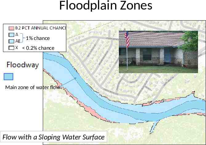
Floodplain Zones 1% chance 0.2% chance Main zone of water flow Flow with a Sloping Water Surface

Types of flow routing Lumped/hydrologic – Flow is calculated as a function of time alone at a particular location – Governed by continuity equation and flow/storage relationship Distributed/hydraulic – Flow is calculated as a function of space and time throughout the system – Governed by continuity and momentum equations 7

Hydrologic Routing Discharge I (t ) Inflow Discharge Transfer Function Q (t ) Outflow I (t ) Inflow Q (t ) Outflow Upstream hydrograph Downstream hydrograph Input, output, and storage are related by continuity equation: dS I (t ) Q (t ) Q and S are unknown dt Storage can be expressed as a function of I(t) or Q(t) or both S f (I , dI dQ , , Q, , ) dt dt For a linear reservoir, S kQ 8

Lumped flow routing Three types 1. Level pool method (Modified Puls) – Storage is nonlinear function of Q 2. Muskingum method – Storage is linear function of I and Q 3. Series of reservoir models – Storage is linear function of Q and its time derivatives 9

S and Q relationships 10

Level pool routing Procedure for calculating outflow hydrograph Q(t) from a reservoir with horizontal water surface, given its inflow hydrograph I(t) and storage-outflow relationship 11

Level pool methodology Discharge dS I (t ) Q(t ) dt Inflow I j 1 Outflow Ij S j 1 ( j 1) t ( j 1) t Sj j t j t dS Q j 1 Qj S j 1 S j t j t ( j 1) t Time t 2S j 1 Storage t Idt Qdt I j 1 I j 2 Q j 1 Q j 2 Q j 1 I j 1 I j Unknown 2S j t Qj Known Need a function relating S j 1 Sj Time 2S Q, and Q t Storage-outflow function 12

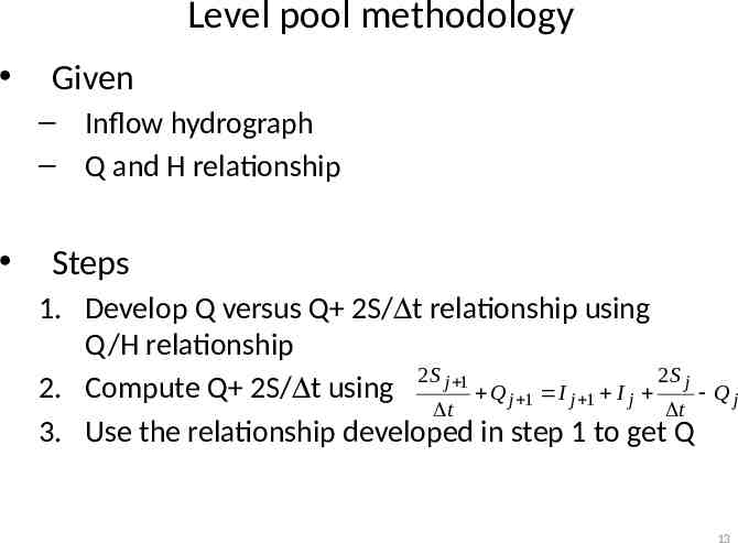
Level pool methodology Given – Inflow hydrograph – Q and H relationship Steps 1. Develop Q versus Q 2S/Dt relationship using Q/H relationship 2 S j 1 2S j 2. Compute Q 2S/Dt using Q j 1 I j 1 I j Qj t t 3. Use the relationship developed in step 1 to get Q 13

Ex. 8.2.1 Given I(t) 0 10 20 30 40 50 60 70 80 90 100 110 120 130 140 150 160 170 180 190 200 210 Inflow (cfs) 0 60 120 180 240 300 360 320 280 240 200 160 120 80 40 0 0 0 0 0 0 0 400 300 Inflow (cfs) Time (min) Given Q/H 200 100 0 0 50 100 150 200 Tim e (m in) 250 Elevation H Discharge Q (ft) (cfs) 0 0 0.5 3 1 8 1.5 17 2 30 2.5 43 3 60 3.5 78 4 97 4.5 117 5 137 5.5 156 6 173 6.5 190 7 205 7.5 218 8 231 8.5 242 9 253 9.5 264 10 275 Area of the reservoir 1 acre, and outlet diameter 5ft 14

Ex. 8.2.1 Step 1 Develop Q versus Q 2S/Dt relationship using Q/H relationship S Area Height 43560 0.5 21,780 ft 3 2S 2 21780 Q 3 75.6 cfs t 10 60 300 250 Outflow Q (cfs) Elevation H Discharge Q Storage S 2S/ t Q 3 (ft ) (ft) (cfs) (cfs) 0 0 0 0 0.5 3 21780 75.6 1 8 43560 153.2 1.5 17 65340 234.8 2 30 87120 320.4 2.5 43 108900 406 3 60 130680 495.6 3.5 78 152460 586.2 4 97 174240 677.8 4.5 117 196020 770.4 5 137 217800 863 5.5 156 239580 954.6 6 173 261360 1044.2 6.5 190 283140 1133.8 7 205 304920 1221.4 7.5 218 326700 1307 8 231 348480 1392.6 8.5 242 370260 1476.2 9 253 392040 1559.8 9.5 264 413820 1643.4 10 275 435600 1727 200 150 100 50 0 0 500 1000 1500 2000 2S/D t Q (cfs) 15

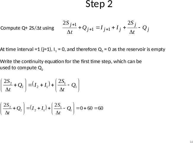
Step 2 Compute Q 2S/Dt using 2 S j 1 t Q j 1 I j 1 I j 2S j t Qj At time interval 1 (j 1), I1 0, and therefore Q1 0 as the reservoir is empty Write the continuity equation for the first time step, which can be used to compute Q2 2S 2 2S Q2 I 2 I1 1 Q1 t t 2S 2 2S Q2 I 2 I1 1 Q1 0 60 60 t t 16

Step 3 300 Use the relationship between 2S/Dt Q versus Q to compute Q 2S 2 Q2 60 t Use the Table/graph created in Step 1 to compute Q What is the value of Q if 2S/Dt Q 60 ? Q 0 (3 0) (60 0) 2.4 cfs (76 0) So Q2 is 2.4 cfs Repeat steps 2 and 3 for j 2, 3, 4 to compute Q3, Q4, Q5 . Outflow Q (cfs) 250 200 150 100 50 0 0 500 1000 1500 2000 2S/D t Q (cfs) Elevation H Discharge Q Storage S 2S/ t Q 3 (ft ) (ft) (cfs) (cfs) 0 0 0 0 0.5 3 21780 75.6 1 8 43560 153.2 1.5 17 65340 234.8 2 30 87120 320.4 2.5 43 108900 406 3 60 130680 495.6 3.5 78 152460 586.2 4 97 174240 677.8 4.5 117 196020 770.4 5 137 217800 863 5.5 156 239580 954.6 6 173 261360 1044.2 6.5 190 283140 1133.8 7 205 304920 1221.4 7.5 218 326700 1307 8 231 348480 1392.6 8.5 242 370260 1476.2 9 253 392040 1559.8 9.5 264 413820 1643.4 10 275 435600 1727 17

Ex. 8.2.1 results 2 S j 1 2S j t Qj 2S j t Q j 2Q j t Q j 1 I j 1 I j 2S j t Qj 18

Ex. 8.2.1 results 12.0 Storage (acre-ft) 10.0 Outflow hydrograph 8.0 6.0 4.0 2.0 0.0 0 20 40 60 80 100 120 140 160 180 200 220 Time (minutes) 400 350 Inflow Peak outflow intersects with the receding limb of the inflow hydrograph Discharge (cfs) 300 250 200 150 Outflow 100 50 0 0 20 40 60 80 100 120 140 160 180 200 220 TIme (minutes) 19

Q/H relationships http://www.wsi.nrcs.usda.gov/products/W2Q/H&H/Tools Models/Sites.html Program for Routing Flow through an NRCS Reservoir 20

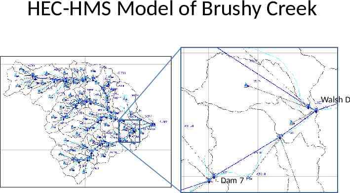
HEC-HMS Model of Brushy Creek Walsh D Dam 7

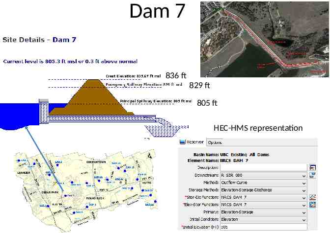
Dam 7, Upper Brushy Creek

Dam 7 836 ft 829 ft 805 ft HEC-HMS representation

Elevation-Storage Curve, Dam 7 Top of Dam, 836 Emergency Spillway, 829

Storage-Discharge Curve, Dam 7 Emergency Top of Spillway, 829 Dam, 836

Dam 7 Hydrologic Simulation

Hydrologic river routing (Muskingum Method) Wedge storage in reach S Prism KQ S Wedge KX ( I Q ) Advancing Flood Wave I Q K travel time of peak through the reach X weight on inflow versus outflow (0 X 0.5) X 0 Reservoir, storage depends on outflow, no wedge X 0.0 - 0.3 Natural stream S KQ KX ( I Q) S K [ XI (1 X )Q] I Q I Q Q Q I Q Receding Flood Wave Q I Q I I I

Muskingum Method (Cont.) S K [ XI (1 X )Q] S j 1 S j K {[ XI j 1 (1 X )Q j 1 ] [ XI j (1 X )Q j ]} Recall: S j 1 S j I j 1 I j 2 t Q j 1 Q j 2 Combine: Q j 1 C1I j 1 C 2 I j C3Q j t t 2 KX 2 K (1 X ) t t 2 KX C2 2 K (1 X ) t 2 K (1 X ) t C3 2 K (1 X ) t C1 If I(t), K and X are known, Q(t) can be calculated using above equations 28

Muskingum - Example Given: – Inflow hydrograph – K 2.3 hr, X 0.15, Dt 1 hour, Initial Q 85 cfs Find: – Outflow hydrograph using Muskingum routing method t 2 KX 1 2 * 2.3 * 0.15 0.0631 2 K (1 X ) t 2 * 2.3(1 0.15) 1 t 2 KX 1 2 * 2.3 * 0.15 C2 0.3442 2 K (1 X ) t 2 * 2.3(1 0.15) 1 2 K (1 X ) t 2 * 2.3 * (1 0.15) 1 C3 0.5927 2 K (1 X ) t 2 * 2.3(1 0.15) 1 C1 Period (hr) 1 2 3 4 5 6 7 8 9 10 11 12 13 14 15 16 17 18 19 20 Inflow (cfs) 93 137 208 320 442 546 630 678 691 675 634 571 477 390 329 247 184 134 108 90 29

Muskingum – Example (Cont.) Q j 1 C1I j 1 C 2 I j C3Q j C1 0.0631, C2 0.3442, C3 0.5927 800 700 Discharge (cfs) 600 500 400 300 Period (hr) 1 2 3 4 5 6 7 8 9 10 11 12 13 14 15 16 17 18 19 20 Inflow (cfs) 93 137 208 320 442 546 630 678 691 675 634 571 477 390 329 247 184 134 108 90 C1Ij 1 0 9 13 20 28 34 40 43 44 43 40 36 30 25 21 16 12 8 7 6 C2Ij 0 32 47 72 110 152 188 217 233 238 232 218 197 164 134 113 85 63 46 37 C3Qj 0 50 54 68 95 138 192 249 301 343 369 380 376 357 324 284 245 202 162 128 Outflow (cfs) 85 91 114 159 233 324 420 509 578 623 642 635 603 546 479 413 341 274 215 170 200 100 0 1 2 3 4 5 6 7 8 9 10 11 12 13 14 15 16 17 18 19 20 Time (hr) 30

HEC-HMS Model of Brushy Creek Walsh D Dam 7

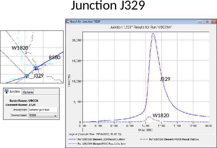
Watershed W1820

Junction J329 W1820 R580 J329 J329 W1820

Reach R580