+ Homework: 2, 4, 6, 10, 12, 14, 28, 30, 34, 36, 38, 42, 50, 52, 54,

Homework: 2, 4, 6, 10, 12, 14, 28, 30, 34, 36, 38, 42, 50, 52, 54, 56, 60, 62, 64 Chapter 7: Sampling Distributions Section 7.1 What is a Sampling Distribution? The Practice of Statistics, 4th edition – For AP* STARNES, YATES, MOORE

Chapter 7 Sampling Distributions 7.1 What is a Sampling Distribution? 7.2 Sample Proportions 7.3 Sample Means

Section 7.1 What Is a Sampling Distribution? Learning Objectives After this section, you should be able to DISTINGUISH between a parameter and a statistic DEFINE sampling distribution DISTINGUISH between population distribution, sampling distribution, and the distribution of sample data DETERMINE whether a statistic is an unbiased estimator of a population parameter DESCRIBE the relationship between sample size and the variability of an estimator

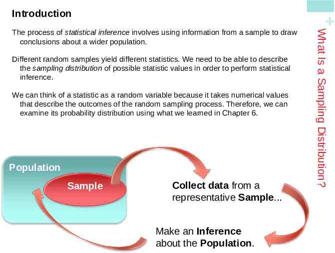
Introduction Different random samples yield different statistics. We need to be able to describe the sampling distribution of possible statistic values in order to perform statistical inference. We can think of a statistic as a random variable because it takes numerical values that describe the outcomes of the random sampling process. Therefore, we can examine its probability distribution using what we learned in Chapter 6. Population Sample Collect data from a representative Sample. Make an Inference about the Population. What Is a Sampling Distribution? The process of statistical inference involves using information from a sample to draw conclusions about a wider population.

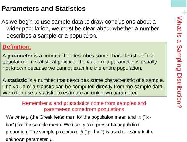
Definition: A parameter is a number that describes some characteristic of the population. In statistical practice, the value of a parameter is usually not known because we cannot examine the entire population. A statistic is a number that describes some characteristic of a sample. The value of a statistic can be computed directly from the sample data. We often use a statistic to estimate an unknown parameter. Remember s and p: statistics come from samples and parameters come from populations We write µ (the Greek letter mu) for the population mean and x (" x bar") for the sample mean. We use p to represent a population proportion. The sample proportion pˆ ("p - hat" ) is used to estimate the unknown parameter p. What Is a Sampling Distribution? As we begin to use sample data to draw conclusions about a wider population, we must be clear about whether a number describes a sample or a population. Parameters and Statistics

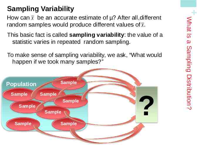
This basic fact is called sampling variability: the value of a statistic varies in repeated random sampling. To make sense of sampling variability, we ask, “What would happen if we took many samples?” Sample Population Sample Sample Sample Sample Sample Sample Sample ? What Is a Sampling Distribution? How can x be an accurate estimate of µ? After all, different random samples would produce different values of x. Sampling Variability

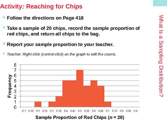
Activity: Reaching for Chips Follow the directions on Page 418 Take a sample of 20 chips, record the sample proportion of red chips, and return all chips to the bag. Report your sample proportion to your teacher. Teacher: Right-click (control-click) on the graph to edit the counts. What Is a Sampling Distribution?

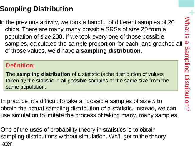
Definition: The sampling distribution of a statistic is the distribution of values taken by the statistic in all possible samples of the same size from the same population. In practice, it’s difficult to take all possible samples of size n to obtain the actual sampling distribution of a statistic. Instead, we can use simulation to imitate the process of taking many, many samples. One of the uses of probability theory in statistics is to obtain sampling distributions without simulation. We’ll get to the theory later. What Is a Sampling Distribution? In the previous activity, we took a handful of different samples of 20 chips. There are many, many possible SRSs of size 20 from a population of size 200. If we took every one of those possible samples, calculated the sample proportion for each, and graphed all of those values, we’d have a sampling distribution. Sampling Distribution

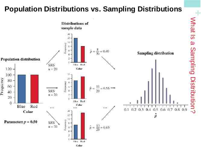
1) The population distribution gives the values of the variable for all the individuals in the population. 2) The distribution of sample data shows the values of the variable for all the individuals in the sample. 3) The sampling distribution shows the statistic values from all the possible samples of the same size from the population. What Is a Sampling Distribution? There are actually three distinct distributions involved when we sample repeatedly and measure a variable of interest. Population Distributions vs. Sampling Distributions

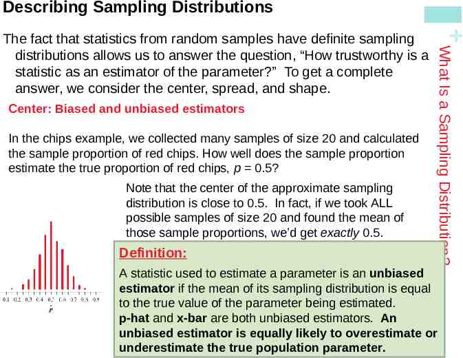
Center: Biased and unbiased estimators In the chips example, we collected many samples of size 20 and calculated the sample proportion of red chips. How well does the sample proportion estimate the true proportion of red chips, p 0.5? Note that the center of the approximate sampling distribution is close to 0.5. In fact, if we took ALL possible samples of size 20 and found the mean of those sample proportions, we’d get exactly 0.5. Definition: What Is a Sampling Distribution? The fact that statistics from random samples have definite sampling distributions allows us to answer the question, “How trustworthy is a statistic as an estimator of the parameter?” To get a complete answer, we consider the center, spread, and shape. Describing Sampling Distributions A statistic used to estimate a parameter is an unbiased estimator if the mean of its sampling distribution is equal to the true value of the parameter being estimated. p-hat and x-bar are both unbiased estimators. An unbiased estimator is equally likely to overestimate or underestimate the true population parameter.

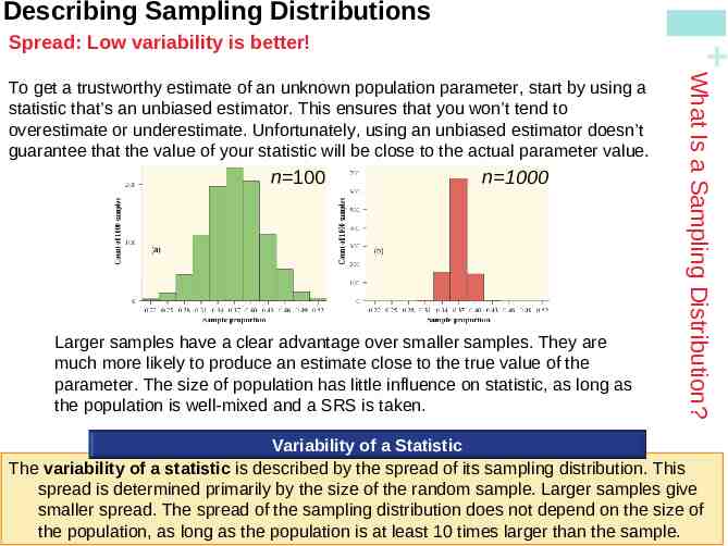
Describing Sampling Distributions Spread: Low variability is better! n 100 n 1000 Larger samples have a clear advantage over smaller samples. They are much more likely to produce an estimate close to the true value of the parameter. The size of population has little influence on statistic, as long as the population is well-mixed and a SRS is taken. What Is a Sampling Distribution? To get a trustworthy estimate of an unknown population parameter, start by using a statistic that’s an unbiased estimator. This ensures that you won’t tend to overestimate or underestimate. Unfortunately, using an unbiased estimator doesn’t guarantee that the value of your statistic will be close to the actual parameter value. Variability of a Statistic The variability of a statistic is described by the spread of its sampling distribution. This spread is determined primarily by the size of the random sample. Larger samples give smaller spread. The spread of the sampling distribution does not depend on the size of the population, as long as the population is at least 10 times larger than the sample.

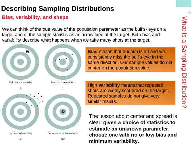
We can think of the true value of the population parameter as the bull’s- eye on a target and of the sample statistic as an arrow fired at the target. Both bias and variability describe what happens when we take many shots at the target. Bias means that our aim is off and we consistently miss the bull’s-eye in the same direction. Our sample values do not center on the population value. High variability means that repeated shots are widely scattered on the target. Repeated samples do not give very similar results. The lesson about center and spread is clear: given a choice of statistics to estimate an unknown parameter, choose one with no or low bias and minimum variability. What Is a Sampling Distribution? Bias, variability, and shape Describing Sampling Distributions

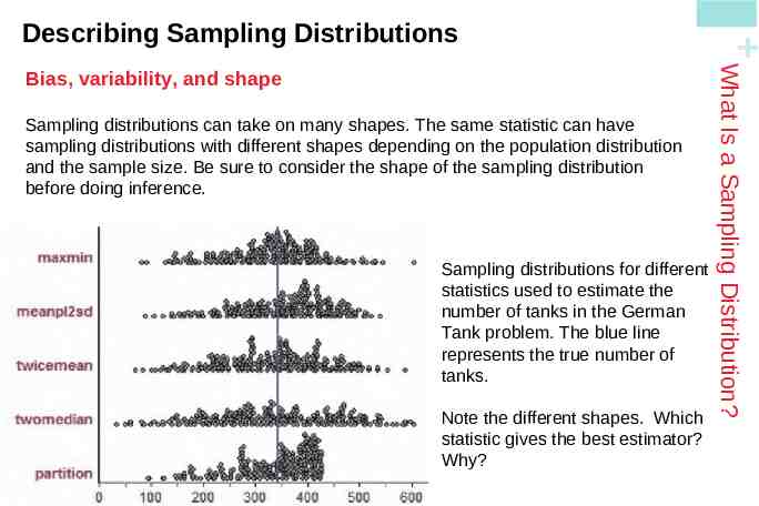
Sampling distributions can take on many shapes. The same statistic can have sampling distributions with different shapes depending on the population distribution and the sample size. Be sure to consider the shape of the sampling distribution before doing inference. Sampling distributions for different statistics used to estimate the number of tanks in the German Tank problem. The blue line represents the true number of tanks. Note the different shapes. Which statistic gives the best estimator? Why? What Is a Sampling Distribution? Bias, variability, and shape Describing Sampling Distributions

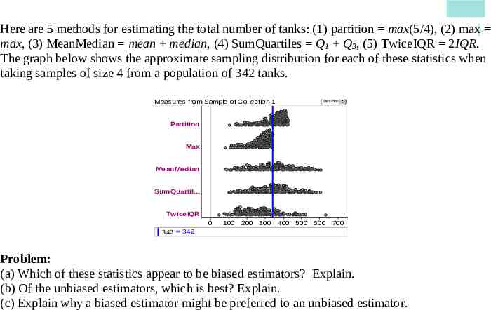
Here are 5 methods for estimating the total number of tanks: (1) partition max(5/4), (2) max max, (3) MeanMedian mean median, (4) SumQuartiles Q1 Q3, (5) TwiceIQR 2IQR. The graph below shows the approximate sampling distribution for each of these statistics when taking samples of size 4 from a population of 342 tanks. Measures from Sample of Collection 1 Dot Plot Partition Max MeanMedian SumQuartil. TwiceIQR 0 100 200 300 400 500 600 700 342 Problem: (a) Which of these statistics appear to be biased estimators? Explain. (b) Of the unbiased estimators, which is best? Explain. (c) Explain why a biased estimator might be preferred to an unbiased estimator.

(a) The statistics Max and TwiceIQR appear to be biased estimators because they are consistently too low. That is, the centers of their sampling distributions appear to be below the correct value of 342. (b) Of the three unbiased statistics, Partition is best since it has the least variability. (c) Even though max is a biased estimator, it often produces estimates very close to the truth. MeanMedian, although unbiased, is quite variable and not close to the true value as often. For example, in 120 of the 250 SRSs, Max produced an estimate within 50 of the true value. However, MeanMedian was this close in only 79 of the 250 SRSs.

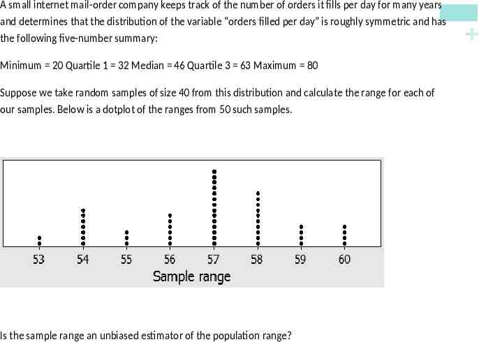
Minimum 20 Quartile 1 32 Median 46 Quartile 3 63 Maximum 80 Suppose we take random samples of size 40 from this distribution and calculate the range for each of our samples. Below is a dotplot of the ranges from 50 such samples. Is the sample range an unbiased estimator of the population range? A small internet mail-order company keeps track of the number of orders it fills per day for many years and determines that the distribution of the variable “orders filled per day” is roughly symmetric and has the following five-number summary:

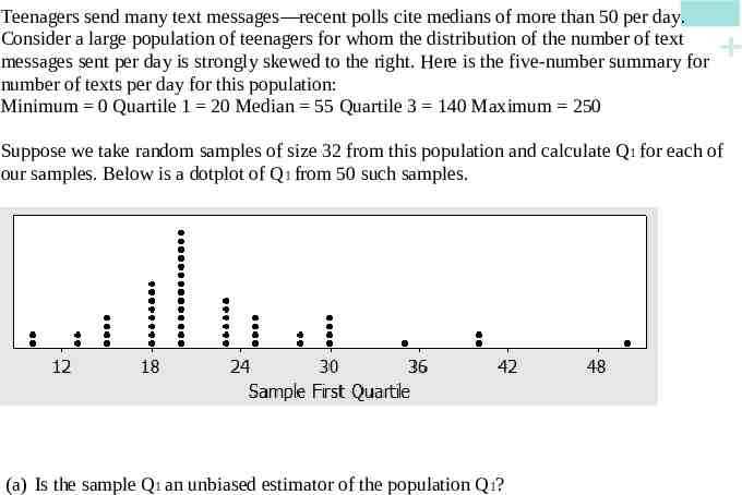
Teenagers send many text messages—recent polls cite medians of more than 50 per day. Consider a large population of teenagers for whom the distribution of the number of text messages sent per day is strongly skewed to the right. Here is the five-number summary for number of texts per day for this population: Minimum 0 Quartile 1 20 Median 55 Quartile 3 140 Maximum 250 Suppose we take random samples of size 32 from this population and calculate Q1 for each of our samples. Below is a dotplot of Q1 from 50 such samples. (a) Is the sample Q1 an unbiased estimator of the population Q1?

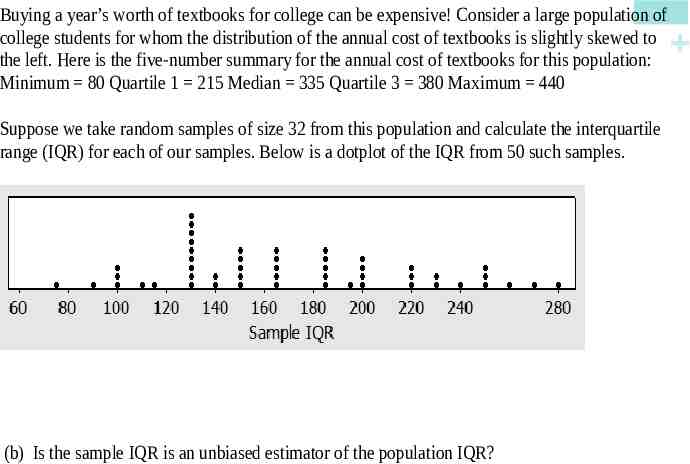
Buying a year’s worth of textbooks for college can be expensive! Consider a large population of college students for whom the distribution of the annual cost of textbooks is slightly skewed to the left. Here is the five-number summary for the annual cost of textbooks for this population: Minimum 80 Quartile 1 215 Median 335 Quartile 3 380 Maximum 440 Suppose we take random samples of size 32 from this population and calculate the interquartile range (IQR) for each of our samples. Below is a dotplot of the IQR from 50 such samples. (b) Is the sample IQR is an unbiased estimator of the population IQR?

Section 7.1 What Is a Sampling Distribution? Summary In this section, we learned that A parameter is a number that describes a population. To estimate an unknown parameter, use a statistic calculated from a sample. The population distribution of a variable describes the values of the variable for all individuals in a population. The sampling distribution of a statistic describes the values of the statistic in all possible samples of the same size from the same population. A statistic can be an unbiased estimator or a biased estimator of a parameter. Bias means that the center (mean) of the sampling distribution is not equal to the true value of the parameter. The variability of a statistic is described by the spread of its sampling distribution. Larger samples give smaller spread. When trying to estimate a parameter, choose a statistic with low or no bias and minimum variability. Don’t forget to consider the shape of the sampling distribution before doing inference.

Looking Ahead In the next Section We’ll learn how to describe and use the sampling distribution of sample proportions. We’ll learn about The sampling distribution of pˆ Using the Normal approximation for pˆ

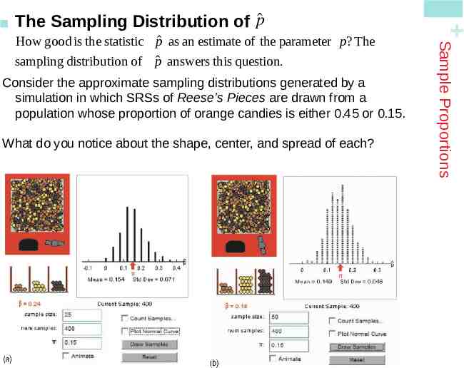
Consider the approximate sampling distributions generated by a Pieces are drawn from a simulation in which SRSs of Reese’s population whose proportion of orange candies is either 0.45 or 0.15. What do you notice about the shape, center, and spread of each? Sample Proportions How good is the statistic pˆ as an estimate of the parameter p? The sampling distributi on of pˆ answers this question. The Sampling Distribution of pˆ

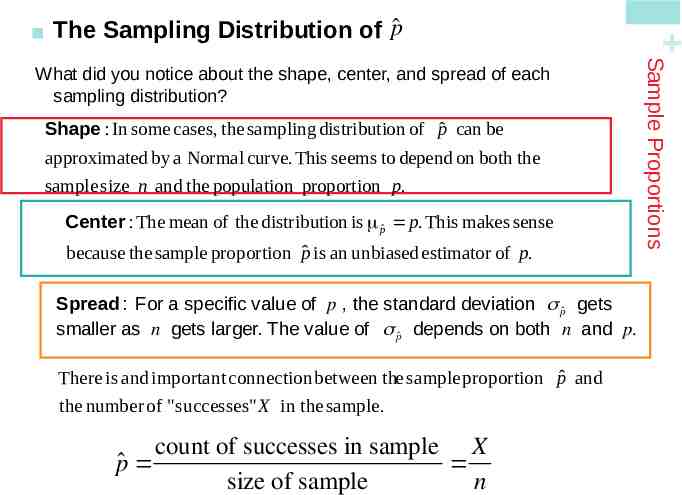
Shape : In some cases, the sampling distribution of pˆ can be approximated by a Normal curve. This seems to depend on both the sample size n and the population proportion p. Center : The mean of the distribution is pˆ p. This makes sense because the sample proportion pˆ is an unbiased estimator of p. Spread : For a specific value of p , the standard deviation pˆ gets smaller as n gets larger. The value of pˆ depends on both n and p. There is and important connection between the sample proportion pˆ and the number of " successes" X in the sample. pˆ count of successes in sample X size of sample n What did you notice about the shape, center, and spread of each sampling distribution? Sample Proportions The Sampling Distribution of pˆ

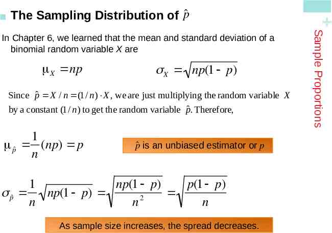
X np(1 p) X np Since pˆ X / n (1 / n) X , we are just multiplying the random variable X by a constant (1 / n) to get the random variable pˆ . Therefore, 1 pˆ (np) p n pˆ is an unbiased estimator or p 1 p(1 p) np(1 p) pˆ np(1 p) 2 n n n As sample size increases, the spread decreases. Sample Proportions In Chapter 6, we learned that the mean and standard deviation of a binomial random variable X are The Sampling Distribution of pˆ

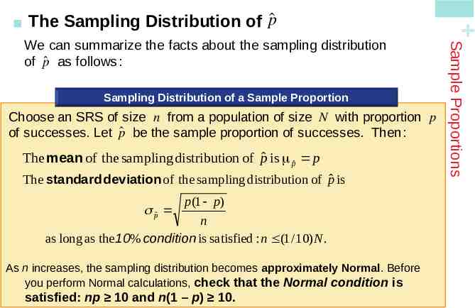
of a Sample Proportion Sampling Distribution Choose an SRS of size n from a population of size N with proportion p of successes. Let pˆ be the sample proportion of successes. Then: The mean of the sampling distribution of pˆ is pˆ p The standard deviation of the sampling distribution of pˆ is p (1 p) n as long as the 10% condition is satisfied : n (1 / 10) N . pˆ As n increases, the sampling distribution becomes approximately Normal. Before you perform Normal calculations, check that the Normal condition is satisfied: np 10 and n(1 – p) 10. We can summarize the facts about the sampling distribution of pˆ as follows : Sample Proportions The Sampling Distribution of pˆ

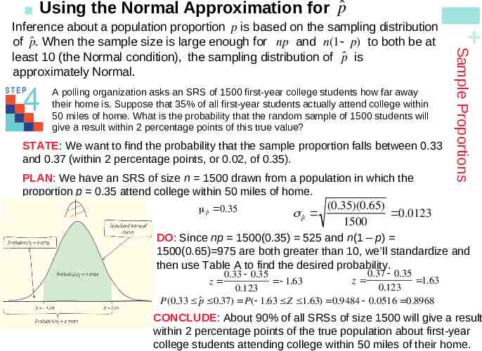
A polling organization asks an SRS of 1500 first-year college students how far away their home is. Suppose that 35% of all first-year students actually attend college within 50 miles of home. What is the probability that the random sample of 1500 students will give a result within 2 percentage points of this true value? STATE: We want to find the probability that the sample proportion falls between 0.33 and 0.37 (within 2 percentage points, or 0.02, of 0.35). PLAN: We have an SRS of size n 1500 drawn from a population in which the proportion p 0.35 attend college within 50 miles of home. pˆ 0.35 pˆ Sample Proportions Inference about a population proportion p is based on the sampling distribution of pˆ . When the sample size is large enough for np and n(1 p) to both be at least 10 (the Normal condition), the sampling distribution of pˆ is approximately Normal. Using the Normal Approximation for pˆ (0.35)(0.65) 0.0123 1500 DO: Since np 1500(0.35) 525 and n(1 – p) 1500(0.65) 975 are both greater than 10, we’ll standardize and then use Table A to find the desired probability. 0.37 0.35 0.33 0.35 z 1.63 1.63 0.123 0.123 P(0.33 pˆ 0.37) P( 1.63 Z 1.63) 0.9484 0.0516 0.8968 z CONCLUDE: About 90% of all SRSs of size 1500 will give a result 2 percentage points of the true population about first-year within college students attending college within 50 miles of their home.

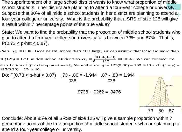
The superintendent of a large school district wants to know what proportion of middle school students in her district are planning to attend a four-year college or university. Suppose that 80% of all middle school students in her district are planning to attend a four-year college or university. What is the probability that a SRS of size 125 will give a result within 7 percentage points of the true value? State: We want to find the probability that the proportion of middle school students who plan to attend a four-year college or university falls between 73% and 87%. That is, P(0.73 p-hat 0.87). Plan: p 0.80. Because the school district is large, we can assume that there are more than 0.80(0.20) 0.036 . We can consider the 125 distribution of p̂ to be approximately Normal since np 125(0.80) 100 10 and n(1 – p) 125(0.20) 25 10. 10(125) 1250 middle school students so pˆ Do: P(0.73 p-hat 0.87) .73 - .80 -1.944 .87 - .80 1.944 .036 .036 .9738 - .0262 .9476 .73 .80 .87 Conclude: About 95% of all SRSs of size 125 will give a sample proportion within 7 percentage points of the true proportion of middle school students who are planning to attend a four-year college or university.

Section 7.2 Sample Proportions Summary In this section, we learned that When we want information about the population proportion p of successes, we ˆ to estimate the unknown often take an SRS and use the sample proportion p parameter p. The sampling distributionof pˆ describes how the statistic varies in all possible samples from the population. The mean of the sampling distribution of pˆ is equal to the population proportion p. That is, pˆ is an unbiased estimator of p. p(1 p) The standard deviation of the sampling distribution of pˆ is pˆ for n an SRS of size n. This formula can be used if the population is at least 10 times as large as the sample (the 10% condition). The standard deviation of pˆ gets smaller as the sample size n gets larger. When the sample size n is larger, the sampling distribution of pˆ is close to a p(1 p) Normal distribution with mean p and standard deviation pˆ . n In practice, use this Normal approximation when both np 10 and n(1 - p) 10 (the Normal condition).

Looking Ahead In the next Section We’ll learn how to describe and use the sampling distribution of sample means. We’ll learn about The sampling distribution of x Sampling from a Normal population The central limit theorem

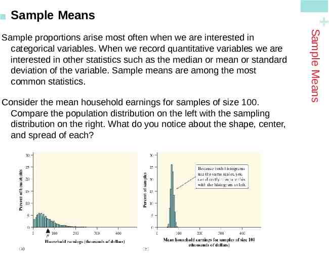
Consider the mean household earnings for samples of size 100. Compare the population distribution on the left with the sampling distribution on the right. What do you notice about the shape, center, and spread of each? Sample Means Sample proportions arise most often when we are interested in categorical variables. When we record quantitative variables we are interested in other statistics such as the median or mean or standard deviation of the variable. Sample means are among the most common statistics. Sample Means

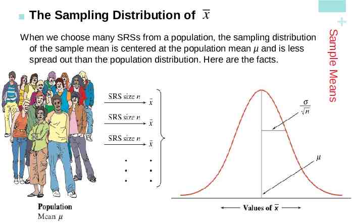
When we choose many SRSs from a population, the sampling distribution of the sample mean is centered at the population mean µ and is less spread out than the population distribution. Here are the facts. Mean and Standard Deviation of the Sampling Distribution of Sample Means Suppose that x is the mean of an SRS of size n drawn from a large population with mean and standard deviation . Then : The mean of the sampling distribution of x is x The standard deviation of the sampling distribution of x is x n as long as the 10% condition is satisfied: n (1/10)N. Note: These facts about the mean and standard deviation ofx are true no matter what shape the population distribution has. x Sample Means The Sampling Distribution of

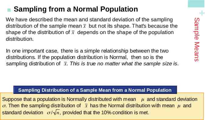
In one important case, there is a simple relationship between the two distributions. If the population distribution is Normal, then so is the sampling distribution of x. This is true no matter what the sample size is. Sample Means We have described the mean and standard deviation of the sampling distribution of the sample mean x but not its shape. That's because the shape of the distribution of x depends on the shape of the population distribution. Sampling from a Normal Population Sampling Distribution of a Sample Mean from a Normal Population Suppose that a population is Normally distributed with mean and standard deviation . Then the sampling distribution of x has the Normal distribution with mean and standard deviation / n, provided that the 10% condition is met.

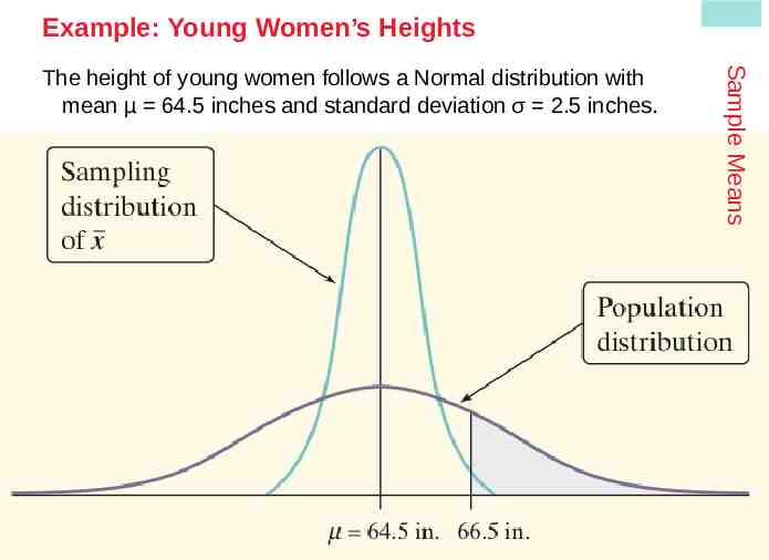
Example: Young Women’s Heights Find the probability that a randomly selected young woman is taller than 66.5 inches. Sample Means The height of young women follows a Normal distribution with mean µ 64.5 inches and standard deviation σ 2.5 inches. Let X the height of a randomly selected young woman. X is N(64.5, 2.5) 66.5 64.5 P(X 66.5) P(Z 0.80) 1 0.7881 0.2119 z 0.80 2.5 The probability of choosing a young woman at random whose height exceeds 66.5 inches is about 0.21. Find the probability that the mean height of an SRS of 10 young women exceeds 66.5 inches. For an SRS of 10 young women, the sampling distribution of their sample mean height will have a mean and standard deviation 2.5 x 64.5 x 0.79 n 10 Since the population distribution is Normal, the sampling distribution will follow an N(64.5, 0.79) distribution. P(x 66.5) P(Z 2.53) 66.5 64.5 z 2.53 1 0.9943 0.0057 0.79 It is very unlikely (less than a 1% chance) that we would choose an SRS of 10 young women whose average height exceeds 66.5 inches.

It is a remarkable fact that as the sample size increases, the distribution of sample means changes its shape: it looks less like that of the population and more like a Normal distribution! When the sample is large enough, the distribution of sample means is very close to Normal, no matter what shape the population distribution has, as long as the population has a finite standard deviation. Sample Means Most population distributions are not Normal. What is the shape of the sampling distribution of sample means when the population distribution isn’t Normal? The Central Limit Theorem Definition: Draw an SRS of size n from any population with mean and finite standard deviation . The central limit theorem (CLT) says that when n is large, the sampling distribution of the sample mean x is approximately Normal. Note: How large a sample size n is needed for the sampling distribution to be close to Normal depends on the shape of the population distribution. More observations are required if the population distribution is far from Normal.

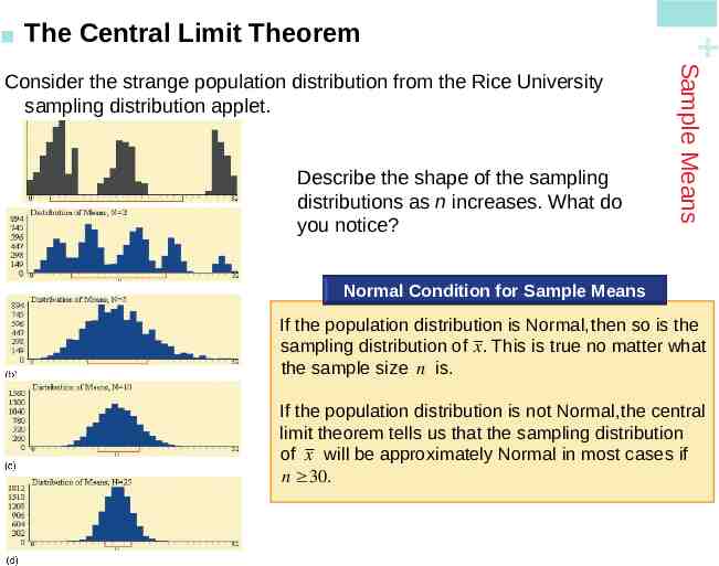
Describe the shape of the sampling distributions as n increases. What do you notice? Sample Means Consider the strange population distribution from the Rice University sampling distribution applet. The Central Limit Theorem Normal Condition for Sample Means If the population distribution is Normal, then so is the sampling distribution of x. This is true no matter what the sample size n is. If the population distribution is not Normal, the central limit theorem tells us that the sampling distribution of x will be approximately Normal in most cases if n 30.

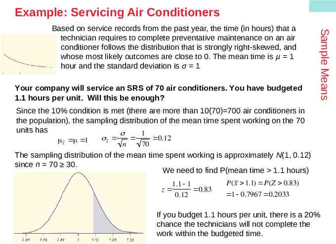
Example: Servicing Air Conditioners Your company will service an SRS of 70 air conditioners. You have budgeted 1.1 hours per unit. Will this be enough? Sample Means Based on service records from the past year, the time (in hours) that a technician requires to complete preventative maintenance on an air conditioner follows the distribution that is strongly right-skewed, and whose most likely outcomes are close to 0. The mean time is µ 1 hour and the standard deviation is σ 1 Since the 10% condition is met (there are more than 10(70) 700 air conditioners in the population), the sampling distribution of the mean time spent working on the 70 units has 1 x 0.12 x 1 n 70 The sampling distribution of the mean time spent working is approximately N(1, 0.12) since n 70 30. We need to find P(mean time 1.1 hours) P(x 1.1) P(Z 0.83) 1.1 1 z 0.83 1 0.7967 0.2033 0.12 If you budget 1.1 hours per unit, there is a 20% chance the technicians will not complete the work within the budgeted time.