Highline Class, BI 348 Basic Business Analytics using Excel Chapter 08

Highline Class, BI 348 Basic Business Analytics using Excel Chapter 08 & 09: Introduction to Linear Programing 1

Topics Covered (Videos): 1. Linear Programming Objective Function Constraint Functions Linear Algebra Solution for Two Decision Variables: Manufacturer Maximizing CM 2. Excel Solver Solution for Two Decision Variables : Manufacturer Maximizing CM Solver Answer Report Solver Sensitivity Report 3. Special Cases: Infeasible, Unbound, Alternative Optimal Solution 4. Excel Solver: Finance Example, Multiple Variables, Maximize Return 5. Excel Solver: Transportation Example, Multiple Variables, Minimize Costs 6. Binary Variable Is Like On On/Off Switch Solver NPV Finance Example, Multiple Variables, Choose When there are Limited Resources 2

Spreadsheet Models (Chapter 7) Models built to solve business related problems. Built with formula inputs, formulas, functions and other Excel features. Decision variables (formula inputs) variables managers have control over. The beauty of such models as that they instantaneous recalculate when formula inputs change. Features such as Data Tables, Goal Seek and Solver can be used to find solutions. 3

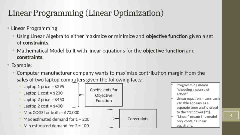
Linear Programming (Linear Optimization) Linear Programming Using Linear Algebra to either maximize or minimize and objective function given a set of constraints. Mathematical Model built with linear equations for the objective function and constraints. Example: Computer manufacturer company wants to maximize contribution margin from the sales of two laptop computers given the following facts: Laptop 1 price 295 Coefficients for Laptop 1 cost 200 Objective Laptop 2 price 450 Function Laptop 2 cost 400 Max COGS for both 70,000 Max estimated demand for 1 200 Min estimated demand for 2 100 Constraints Programming means “choosing a course of action”. Linear equation means each variable appears as a separate term and is raised to the first power ( 1). “Linear” means the model only contains linear equations. 4

Steps in Building Linear Program 1. Read problem carefully and take notes. Gather necessary data. 2. List variables and state objective (goal). State Objective: max or min. Define Decision Variables Variables management has control over. List Parameters Assumptions, Formula Inputs, Coefficients. List Constraints. 3. Define Linear Equations for: Objective Function Formula to find optimal solution for, max or min. Formula that uses Decision Variables as formula inputs. Formula will have coefficients for each decision variable. 3. Define Linear Equations for: Constraint Functions Formulas that place limitations on finding an optimal solution. Restrictions that limit the outcomes of the decision variables. Formula that uses Decision Variables as formula inputs. The amount of the constraint will be the Right-Side of the constraint linear inequality. 4. Solve on paper using algebra 5. Solve using Excel Solver 5

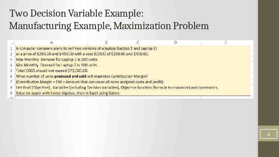
Two Decision Variable Example: Manufacturing Example, Maximization Problem 6

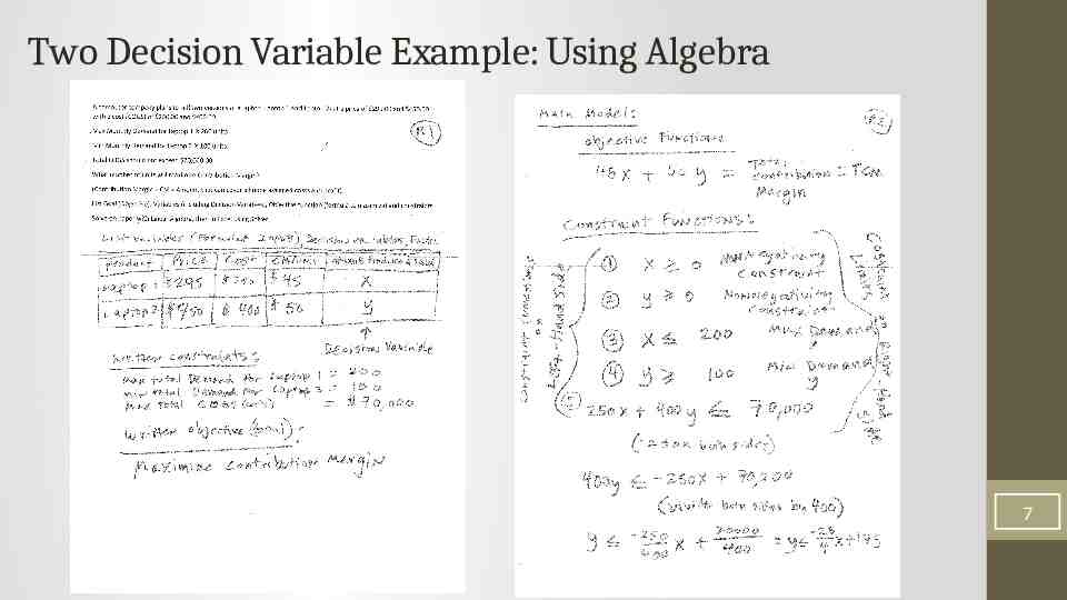
Two Decision Variable Example: Using Algebra 7

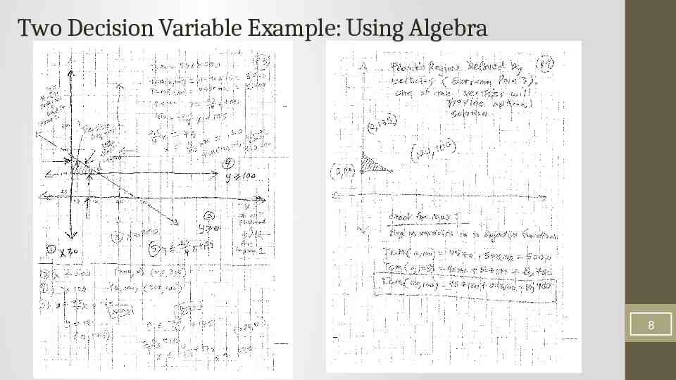
Two Decision Variable Example: Using Algebra 8

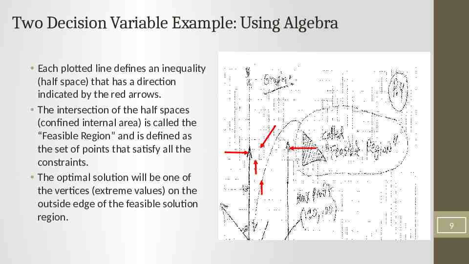
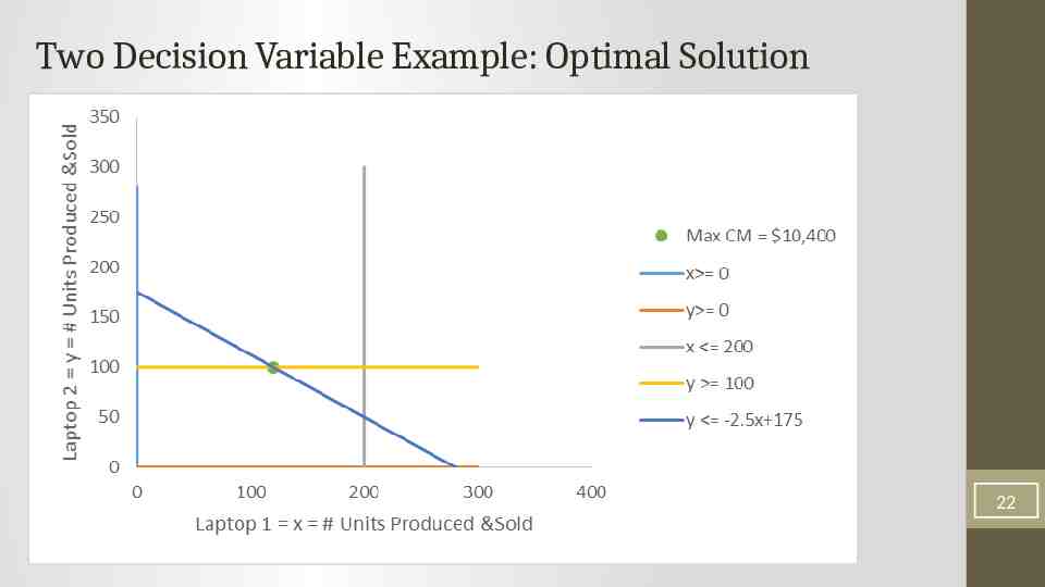
Two Decision Variable Example: Using Algebra Each plotted line defines an inequality (half space) that has a direction indicated by the red arrows. The intersection of the half spaces (confined internal area) is called the “Feasible Region” and is defined as the set of points that satisfy all the constraints. The optimal solution will be one of the vertices (extreme values) on the outside edge of the feasible solution region. 9

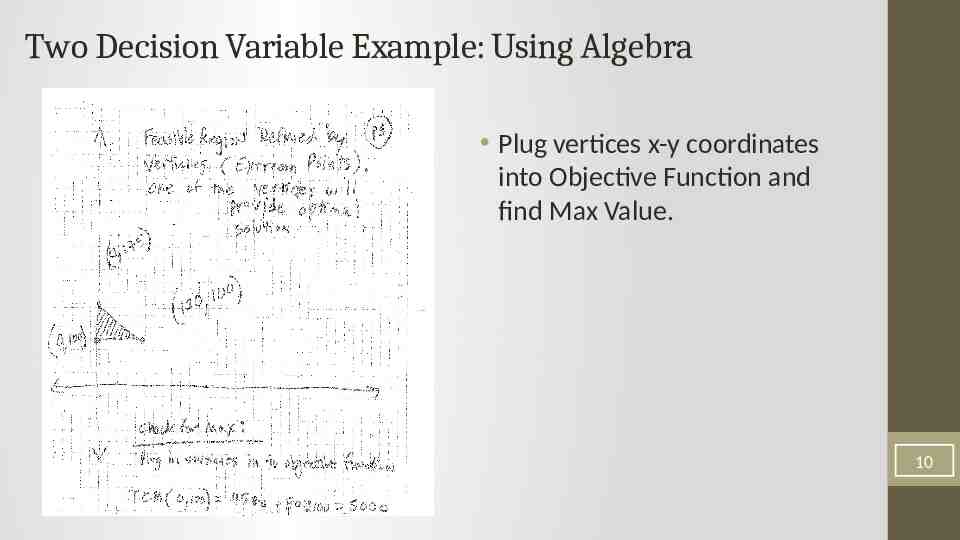
Two Decision Variable Example: Using Algebra Plug vertices x-y coordinates into Objective Function and find Max Value. 10

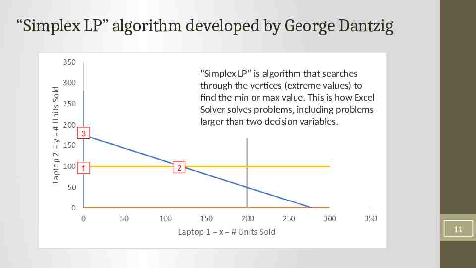
“Simplex LP” algorithm developed by George Dantzig “Simplex LP” is algorithm that searches through the vertices (extreme values) to find the min or max value. This is how Excel Solver solves problems, including problems larger than two decision variables. 3 1 2 11

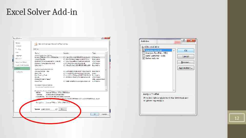
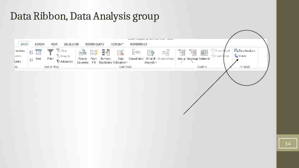
Excel Solver Add-in 12

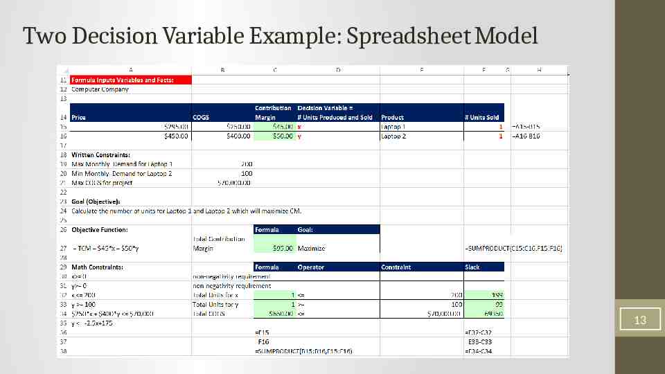
Two Decision Variable Example: Spreadsheet Model 13

Data Ribbon, Data Analysis group 14

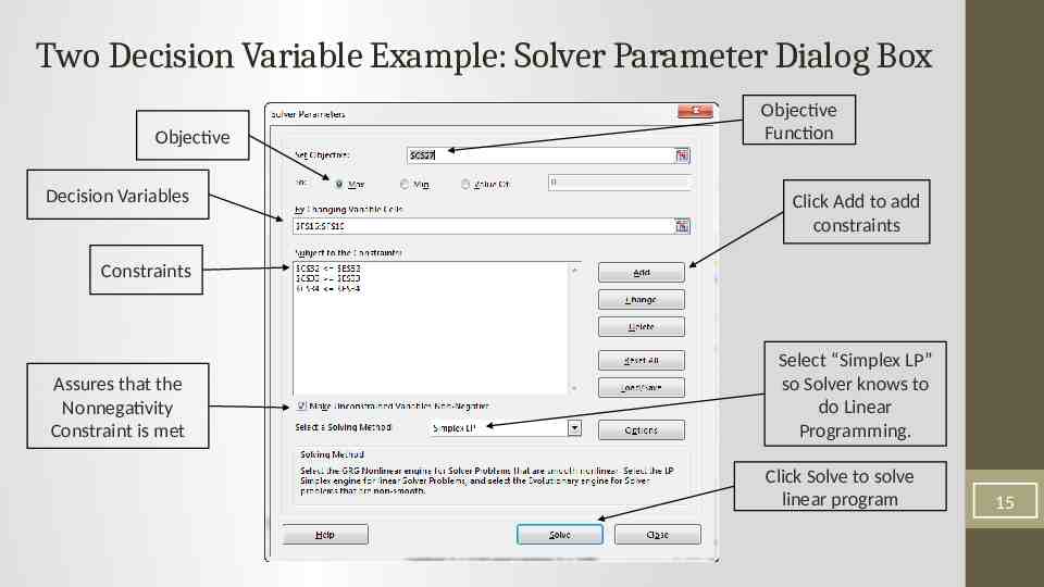
Two Decision Variable Example: Solver Parameter Dialog Box Objective Decision Variables Objective Function Click Add to add constraints Constraints Assures that the Nonnegativity Constraint is met Select “Simplex LP” so Solver knows to do Linear Programming. Click Solve to solve linear program 15

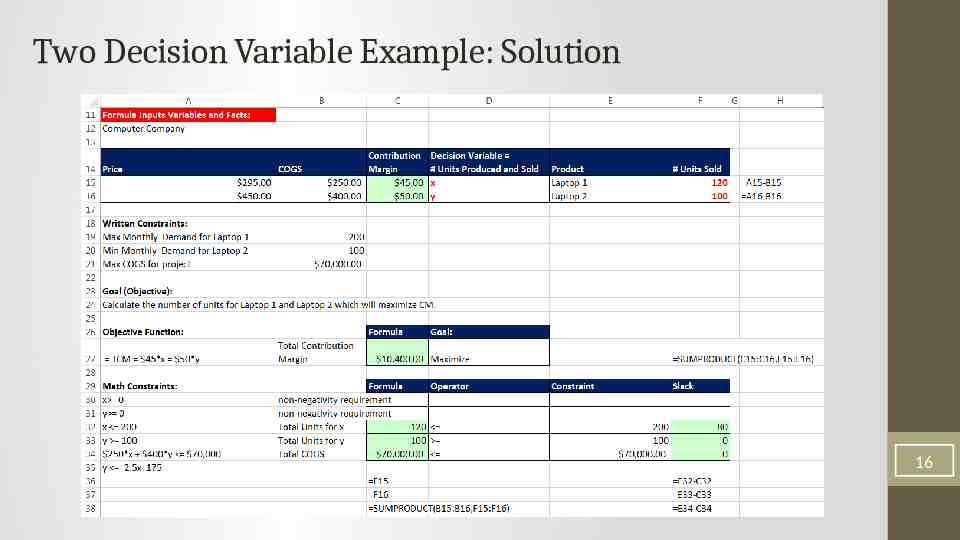
Two Decision Variable Example: Solution 16

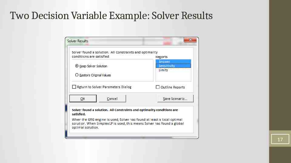
Two Decision Variable Example: Solver Results 17

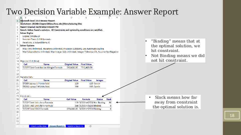
Two Decision Variable Example: Answer Report “Binding” means that at the optimal solution, we hit constraint. Not Binding means we did not hit constraint. Slack means how far away from constraint the optimal solution is. 18

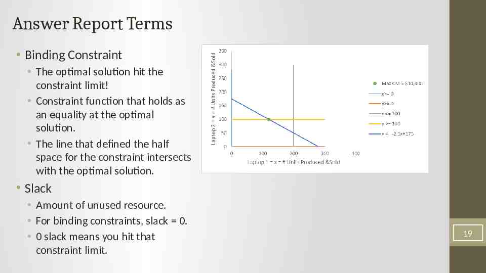
Answer Report Terms Binding Constraint The optimal solution hit the constraint limit! Constraint function that holds as an equality at the optimal solution. The line that defined the half space for the constraint intersects with the optimal solution. Slack Amount of unused resource. For binding constraints, slack 0. 0 slack means you hit that constraint limit. 19

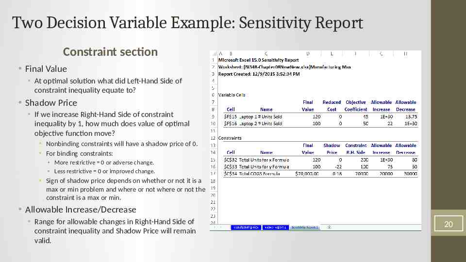
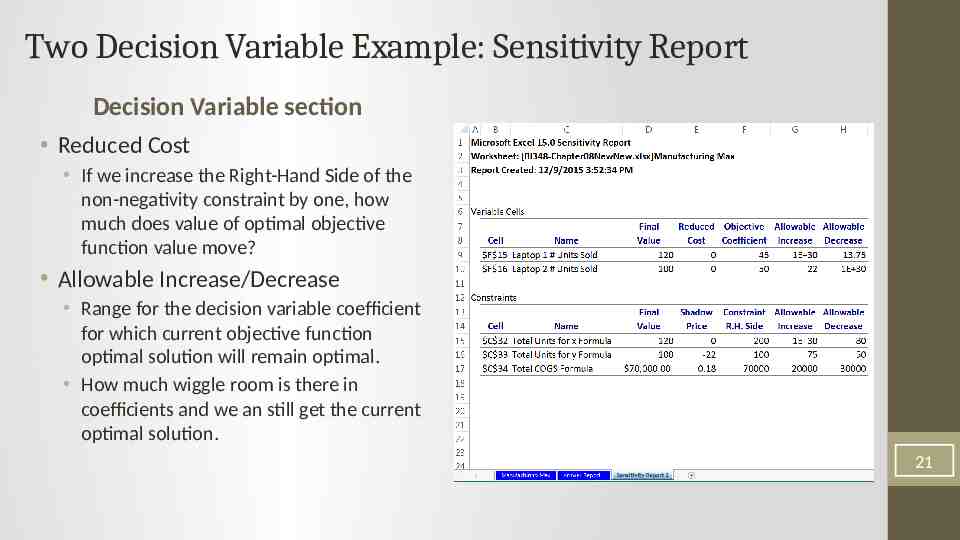
Two Decision Variable Example: Sensitivity Report Constraint section Final Value At optimal solution what did Left-Hand Side of constraint inequality equate to? Shadow Price If we increase Right-Hand Side of constraint inequality by 1, how much does value of optimal objective function move? Nonbinding constraints will have a shadow price of 0. For binding constraints: More restrictive 0 or adverse change. Less restrictive 0 or improved change. Sign of shadow price depends on whether or not it is a max or min problem and where or not where or not the constraint is a max or min. Allowable Increase/Decrease Range for allowable changes in Right-Hand Side of constraint inequality and Shadow Price will remain valid. 20

Two Decision Variable Example: Sensitivity Report Decision Variable section Reduced Cost If we increase the Right-Hand Side of the non-negativity constraint by one, how much does value of optimal objective function value move? Allowable Increase/Decrease Range for the decision variable coefficient for which current objective function optimal solution will remain optimal. How much wiggle room is there in coefficients and we an still get the current optimal solution. 21

Two Decision Variable Example: Optimal Solution 22

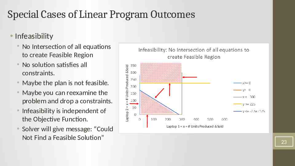
Special Cases of Linear Program Outcomes No Intersection of all equations to create Feasible Region No solution satisfies all constraints. Maybe the plan is not feasible. Maybe you can reexamine the problem and drop a constraints. Infeasibility is independent of the Objective Function. Solver will give message: “Could Not Find a Feasible Solution” Laptop 2 x # Units Produced &Sold Infeasibility Laptop 1 x # Units Produced &Sold 23

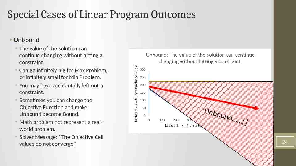
Special Cases of Linear Program Outcomes The value of the solution can continue changing without hitting a constraint. Can go infinitely big for Max Problem, or infinitely small for Min Problem. You may have accidentally left out a constraint. Sometimes you can change the Objective Function and make Unbound become Bound. Math problem not represent a realworld problem. Solver Message: “The Objective Cell values do not converge”. Laptop 2 x # Units Produced &Sold Unbound Unbo und Laptop 1 x # Units Produced &Sold 24

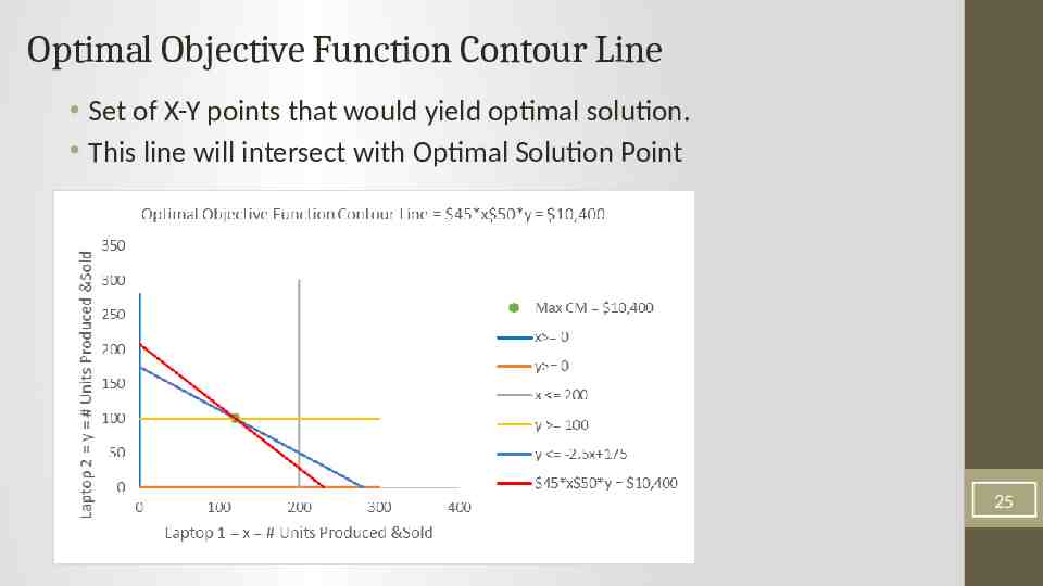
Optimal Objective Function Contour Line Set of X-Y points that would yield optimal solution. This line will intersect with Optimal Solution Point 25

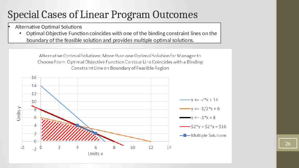
Special Cases of Linear Program Outcomes Alternative Optimal Solutions Optimal Objective Function coincides with one of the binding constraint lines on the boundary of the feasible solution and provides multiple optimal solutions. 26

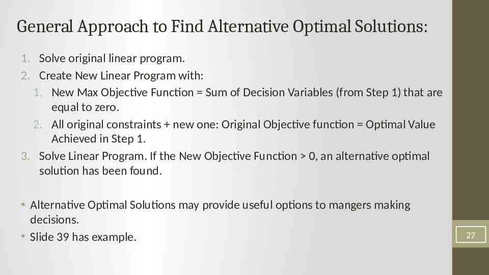
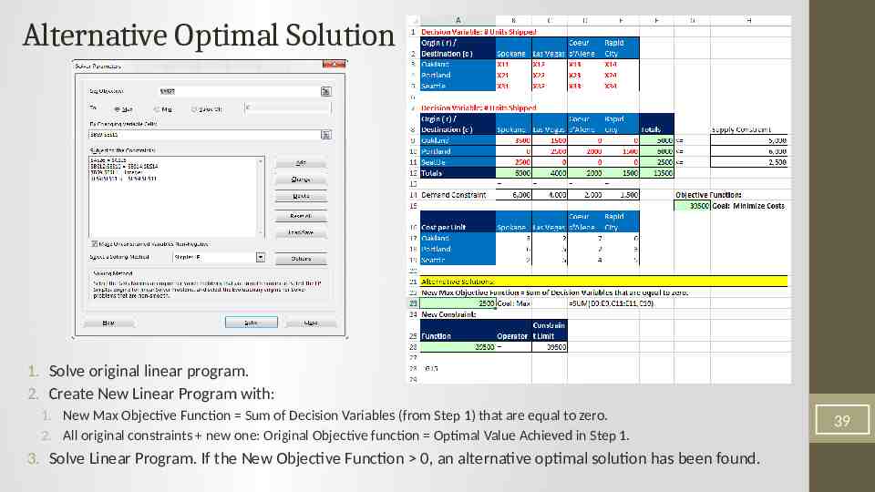
General Approach to Find Alternative Optimal Solutions: 1. Solve original linear program. 2. Create New Linear Program with: 1. New Max Objective Function Sum of Decision Variables (from Step 1) that are equal to zero. 2. All original constraints new one: Original Objective function Optimal Value Achieved in Step 1. 3. Solve Linear Program. If the New Objective Function 0, an alternative optimal solution has been found. Alternative Optimal Solutions may provide useful options to mangers making decisions. Slide 39 has example. 27

Liner Programming Assumptions* 1. Proportionality — the effect of a decision variable in any one equation is proportional to a constant quantity. 2. Additivity — the combined effect of the decision variables in any one equation is the algebraic sum of their individual weighted effects. (The weighting, of course, is due to the proportionality constants.) 3. Divisibility — the decision variables can take on fractional (non-integer) values. 4. Certainty — all model parameters are known constants. 28 *quoted from: https://sites.google.com/site/decisionmodeling/Home/mp/lp/assmp

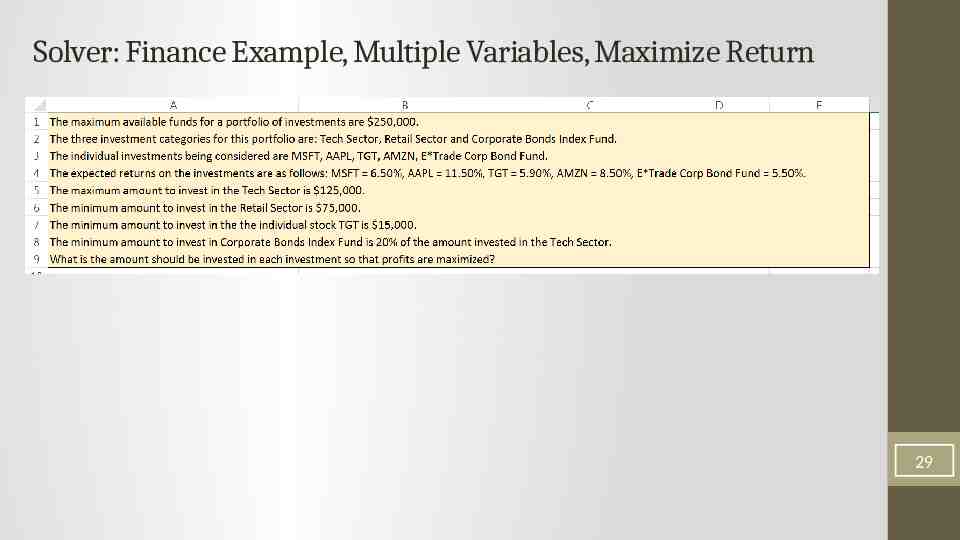
Solver: Finance Example, Multiple Variables, Maximize Return 29

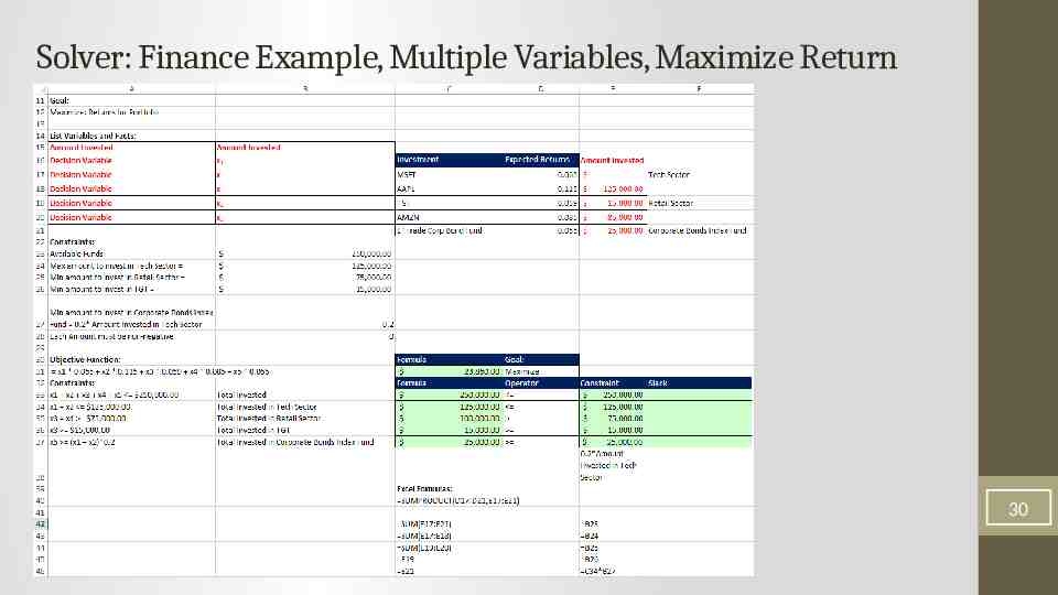
Solver: Finance Example, Multiple Variables, Maximize Return 30

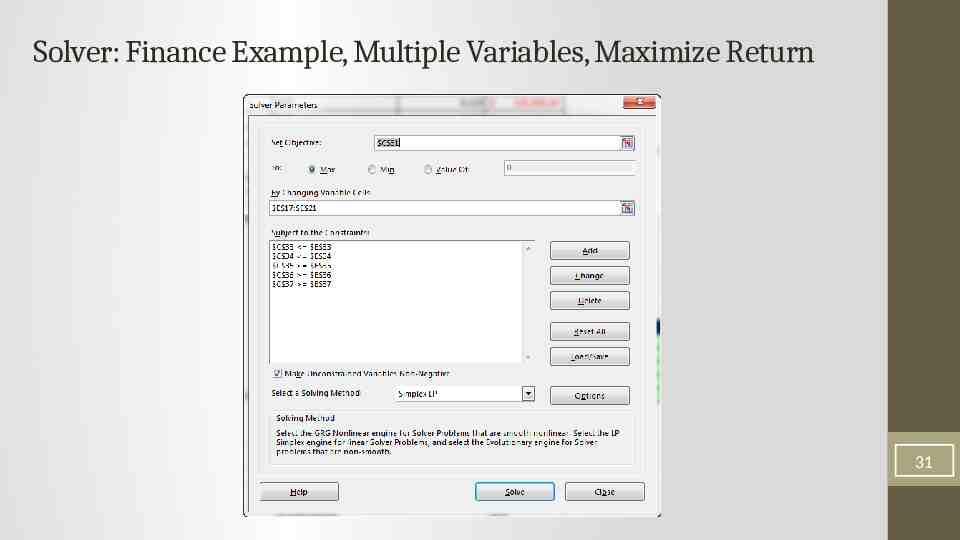
Solver: Finance Example, Multiple Variables, Maximize Return 31

Integer Liner Optimization Rounding to find Integer Solution If you have an integer variable, running the model through Solver may yield noninteger answers. If rounding is insignificant, then rounding is okay. If rounding significantly changes the number so that it because an unacceptable number or puts the answer outside the feasible region, then we need to add an “integer constraint”. Rounding an integer solution is a trial and error process. Each rounding effort must: Checked to see if it is in feasible range. Check against past objective function results. The trial and error process may not yield the optimal solution. To avoid rounding manually, we can require that our Linear Program deliver an integer solution. 32

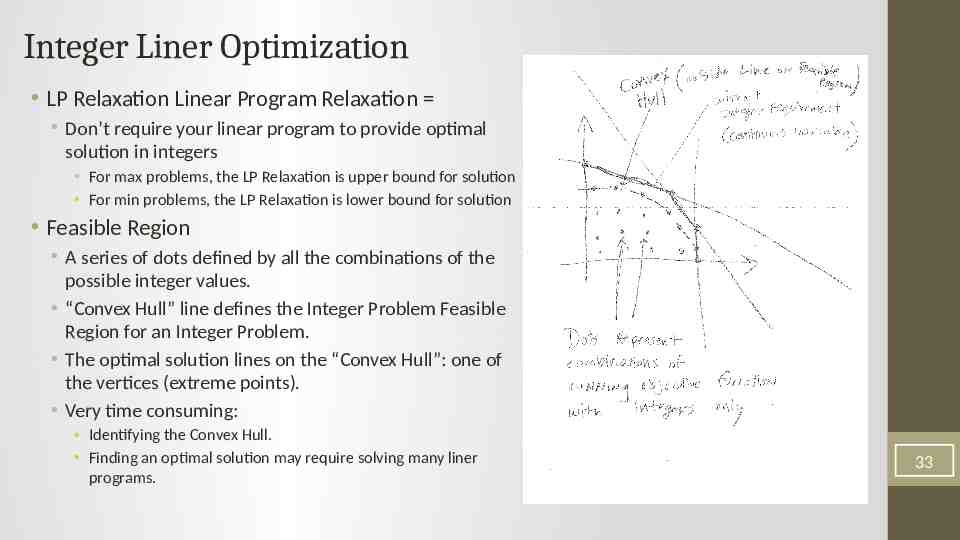
Integer Liner Optimization LP Relaxation Linear Program Relaxation Don’t require your linear program to provide optimal solution in integers For max problems, the LP Relaxation is upper bound for solution For min problems, the LP Relaxation is lower bound for solution Feasible Region A series of dots defined by all the combinations of the possible integer values. “Convex Hull” line defines the Integer Problem Feasible Region for an Integer Problem. The optimal solution lines on the “Convex Hull”: one of the vertices (extreme points). Very time consuming: Identifying the Convex Hull. Finding an optimal solution may require solving many liner programs. 33

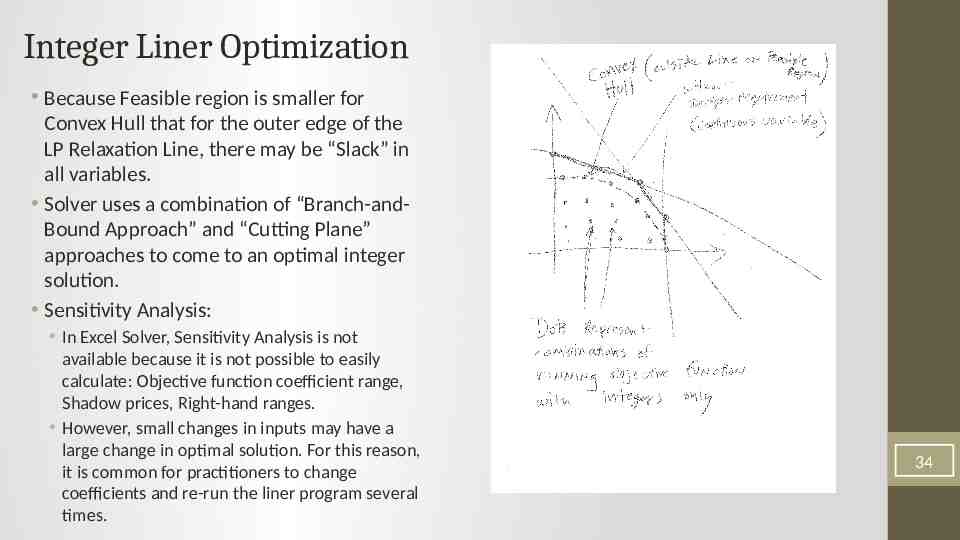
Integer Liner Optimization Because Feasible region is smaller for Convex Hull that for the outer edge of the LP Relaxation Line, there may be “Slack” in all variables. Solver uses a combination of “Branch-andBound Approach” and “Cutting Plane” approaches to come to an optimal integer solution. Sensitivity Analysis: In Excel Solver, Sensitivity Analysis is not available because it is not possible to easily calculate: Objective function coefficient range, Shadow prices, Right-hand ranges. However, small changes in inputs may have a large change in optimal solution. For this reason, it is common for practitioners to change coefficients and re-run the liner program several times. 34

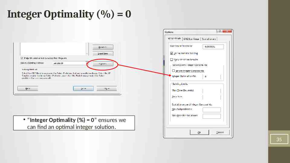
Integer Optimality (%) 0 “Integer Optimality (%) 0” ensures we can find an optimal integer solution. 35

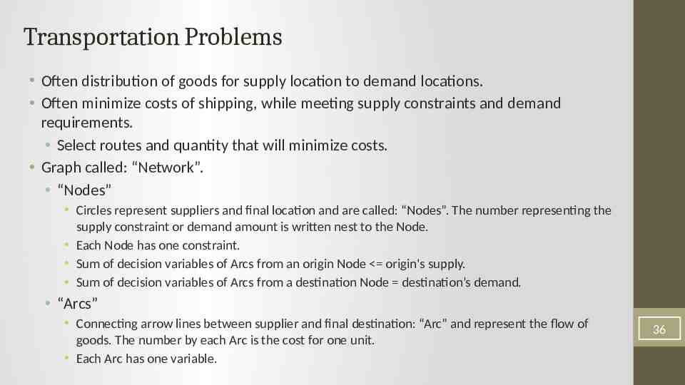
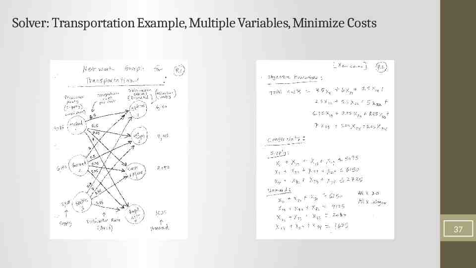
Transportation Problems Often distribution of goods for supply location to demand locations. Often minimize costs of shipping, while meeting supply constraints and demand requirements. Select routes and quantity that will minimize costs. Graph called: “Network”. “Nodes” Circles represent suppliers and final location and are called: “Nodes”. The number representing the supply constraint or demand amount is written nest to the Node. Each Node has one constraint. Sum of decision variables of Arcs from an origin Node origin's supply. Sum of decision variables of Arcs from a destination Node destination’s demand. “Arcs” Connecting arrow lines between supplier and final destination: “Arc” and represent the flow of goods. The number by each Arc is the cost for one unit. Each Arc has one variable. 36

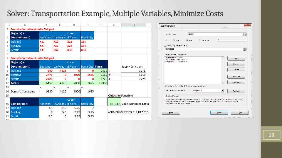
Solver: Transportation Example, Multiple Variables, Minimize Costs 37

Solver: Transportation Example, Multiple Variables, Minimize Costs 38

Alternative Optimal Solution 1. Solve original linear program. 2. Create New Linear Program with: 1. New Max Objective Function Sum of Decision Variables (from Step 1) that are equal to zero. 2. All original constraints new one: Original Objective function Optimal Value Achieved in Step 1. 3. Solve Linear Program. If the New Objective Function 0, an alternative optimal solution has been found. 39

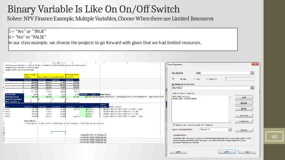
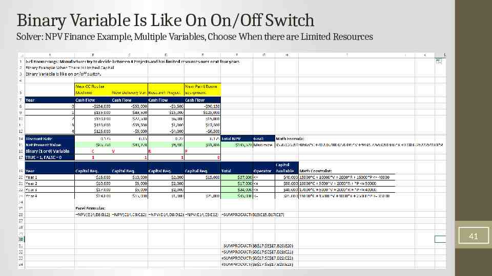
Binary Variable Is Like On On/Off Switch Solver: NPV Finance Example, Multiple Variables, Choose When there are Limited Resources 1 “Yes” or “TRUE” 0 “No” or “FALSE” In our class example, we choose the projects to go forward with given that we had limited resources. 40

Binary Variable Is Like On On/Off Switch Solver: NPV Finance Example, Multiple Variables, Choose When there are Limited Resources 41