Fixed Exchange Rates and Foreign Exchange Intervention Chapter

June 22, 2023

45 Less than a minute

58 Slides815.05 KB

Save Document

Fixed Exchange Rates and Foreign Exchange Intervention Chapter 18 Krugman and Obstfeld 9e ECO41 International Economics Udayan Roy

Why Study Fixed Exchange Rates? Four reasons to study fixed exchange rates: – Managed floating – Regional currency arrangements – Developing countries and countries in transition – Lessons of the past for the future

Central Bank Intervention and the Money Supply Any central bank purchase of assets automatically results in an increase in the domestic money supply (Ms ). – Example: If the US central bank (“The Fed”) buys some financial asset, it must pay for it with newly printed dollars. Therefore, the US money supply must increase.

Central Bank Intervention and the Money Supply Any central bank sale of assets automatically causes a decrease in the money supply (Ms ). – Example: If the Fed sells some financial asset, the dollars paid by the buyer will no longer be in circulation. Therefore, the US money supply must decrease. In short, the central bank’s reserves of financial assets moves in the same direction as its money supply.

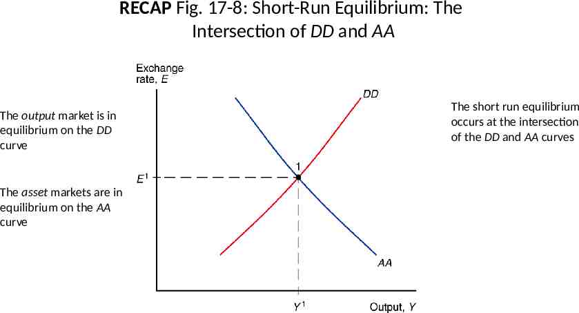
RECAP Fig. 17-8: Short-Run Equilibrium: The Intersection of DD and AA The output market is in equilibrium on the DD curve The asset markets are in equilibrium on the AA curve The short run equilibrium occurs at the intersection of the DD and AA curves

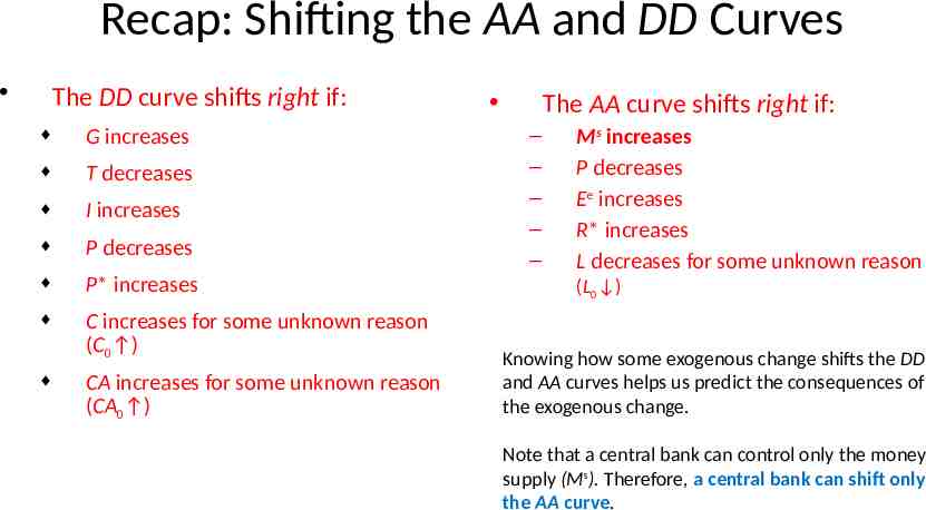
Recap: Shifting the AA and DD Curves The DD curve shifts right if: G increases T decreases I increases P decreases P* increases C increases for some unknown reason (C0 ) CA increases for some unknown reason (CA0 ) The AA curve shifts right if: – – – – – Ms increases P decreases Ee increases R* increases L decreases for some unknown reason (L0 ) Knowing how some exogenous change shifts the DD and AA curves helps us predict the consequences of the exogenous change. Note that a central bank can control only the money supply (Ms). Therefore, a central bank can shift only the AA curve.

SHORT-RUN MACROECONOMICS UNDER FIXED EXCHANGE RATES

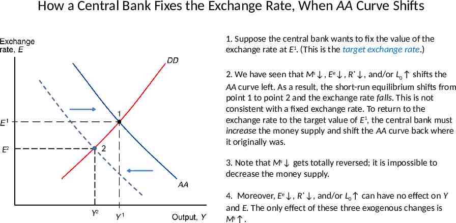
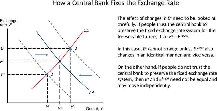
How a Central Bank Fixes the Exchange Rate, When AA Curve Shifts 1. Suppose the central bank wants to fix the value of the exchange rate at E1. (This is the target exchange rate.) 2 E2 2. We have seen that Ms , Ee , R* , and/or L0 shifts the AA curve left. As a result, the short-run equilibrium shifts from point 1 to point 2 and the exchange rate falls. This is not consistent with a fixed exchange rate. To return to the exchange rate to the target value of E1, the central bank must increase the money supply and shift the AA curve back where it originally was. 3. Note that Ms gets totally reversed; it is impossible to decrease the money supply. Y2 4. Moreover, Ee , R* , and/or L0 can have no effect on Y and E. The only effect of these three exogenous changes is Ms .

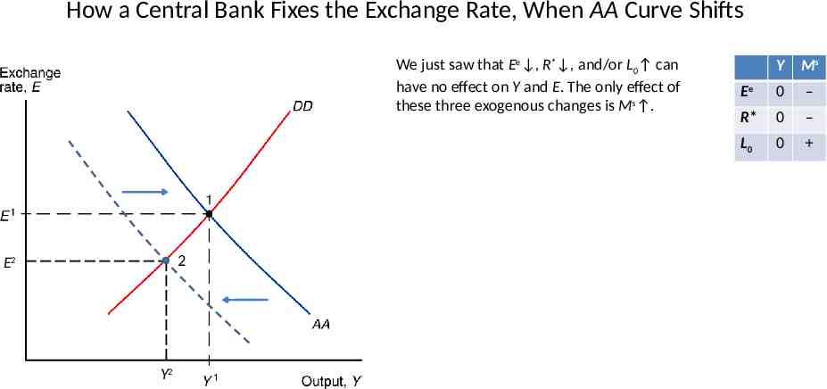
How a Central Bank Fixes the Exchange Rate, When AA Curve Shifts We just saw that Ee , R* , and/or L0 can have no effect on Y and E. The only effect of these three exogenous changes is Ms . 2 E2 Y2 Y Ms Ee 0 – R* 0 – L0 0

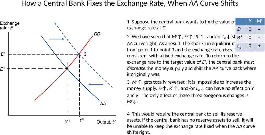
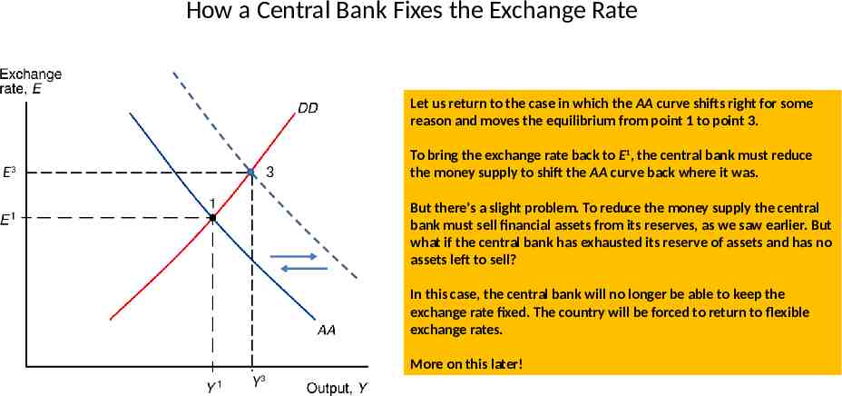
How a Central Bank Fixes the Exchange Rate, When AA Curve Shifts 3 E3 1. Suppose the central bank wants to fix the value of the Y Ms exchange rate at E1. Ee 0 – 2. We have seen that Ms , Ee , R* , and/or L0 shifts R* the0 – AA curve right. As a result, the short-run equilibrium shifts L0 0 from point 1 to point 3 and the exchange rate rises. This is not consistent with a fixed exchange rate. To return to the exchange rate to the target value of E1, the central bank must decrease the money supply and shift the AA curve back where it originally was. 3. Ms gets totally reversed; it is impossible to increase the money supply. Ee , R* , and/or L0 can have no effect on Y and E. The only effect of these three exogenous changes is Ms . Y3 4. This would require the central bank to sell its reserve assets. If the central bank has no reserve assets to sell, it will be unable to keep the exchange rate fixed when the AA curve shifts right.

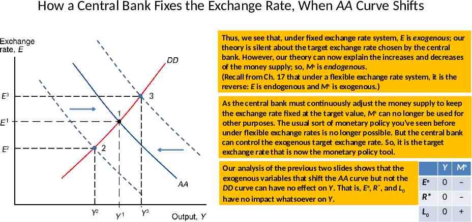
How a Central Bank Fixes the Exchange Rate, When AA Curve Shifts Thus, we see that, under fixed exchange rate system, E is exogenous; our theory is silent about the target exchange rate chosen by the central bank. However, our theory can now explain the increases and decreases of the money supply; so, Ms is endogenous. (Recall from Ch. 17 that under a flexible exchange rate system, it is the reverse: E is endogenous and Ms is exogenous.) 3 E3 2 E2 As the central bank must continuously adjust the money supply to keep the exchange rate fixed at the target value, Ms can no longer be used for other purposes. The usual sort of monetary policy you’ve seen before under flexible exchange rates is no longer possible. But the central bank can control the exogenous target exchange rate. So, it is the target exchange rate that is now the monetary policy tool. Our analysis of the previous two slides shows that the exogenous variables that shift the AA curve but not the DD curve can have no effect on Y. That is, Ee, R*, and L0 have no impact whatsoever on Y. Y2 Y3 Y Ms Ee 0 – R* 0 – L0 0

How a Central Bank Fixes the Exchange Rate Let us return to the case in which the AA curve shifts right for some reason and moves the equilibrium from point 1 to point 3. 3 E3 To bring the exchange rate back to E1, the central bank must reduce the money supply to shift the AA curve back where it was. But there’s a slight problem. To reduce the money supply the central bank must sell financial assets from its reserves, as we saw earlier. But what if the central bank has exhausted its reserve of assets and has no assets left to sell? In this case, the central bank will no longer be able to keep the exchange rate fixed. The country will be forced to return to flexible exchange rates. More on this later! Y 3

How a Central Bank Fixes the Exchange Rate The effect of changes in Ee need to be looked at carefully. If people trust the central bank to preserve the fixed exchange rate system for the foreseeable future, then Ee ETarget. 3 E3 On the other hand, if people do not trust the central bank to preserve the fixed exchange rate system, then Ee and ETarget need not be equal and may move independently. 2 E2 Y2 In this case, Ee cannot change unless ETarget also changes in an identical manner, and vice versa. Y3

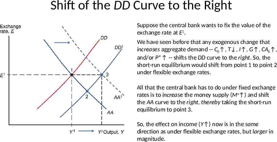
Shift of the DD Curve to the Right Suppose the central bank wants to fix the value of the exchange rate at E1. DD 2 3 2 AA2 Y3 We have seen before that any exogenous change that increases aggregate demand -- C0 , T , I , G , CA0 , and/or P* -- shifts the DD curve to the right. So, the short-run equilibrium would shift from point 1 to point 2 under flexible exchange rates. All that the central bank has to do under fixed exchange rates is to increase the money supply (Ms ) and shift the AA curve to the right, thereby taking the short-run equilibrium to point 3. So, the effect on income (Y ) now is in the same direction as under flexible exchange rates, but larger in magnitude.

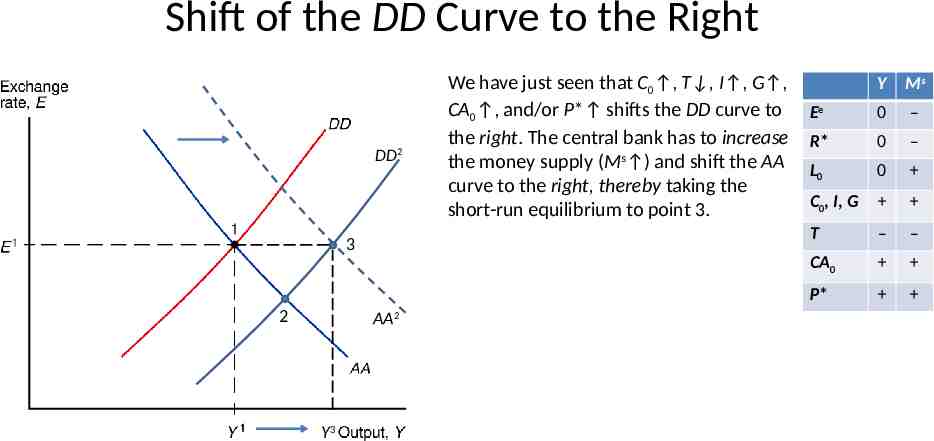
Shift of the DD Curve to the Right DD 2 3 2 AA2 Y3 We have just seen that C0 , T , I , G , CA0 , and/or P* shifts the DD curve to the right. The central bank has to increase the money supply (Ms ) and shift the AA curve to the right, thereby taking the short-run equilibrium to point 3. Y Ms Ee 0 – R* 0 – L0 0 C0, I, G T – – CA0 P*

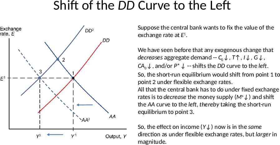
Shift of the DD Curve to the Left DD2 Suppose the central bank wants to fix the value of the exchange rate at E1. We have seen before that any exogenous change that decreases aggregate demand -- C0 , T , I , G , CA0 , and/or P* -- shifts the DD curve to the left. So, the short-run equilibrium would shift from point 1 to point 2 under flexible exchange rates. All that the central bank has to do under fixed exchange rates is to decrease the money supply (Ms ) and shift the AA curve to the left, thereby taking the short-run equilibrium to point 3. 2 3 AA2 Y3 So, the effect on income (Y ) now is in the same direction as under flexible exchange rates, but larger in magnitude.

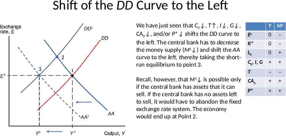
Shift of the DD Curve to the Left DD2 2 3 AA2 Y3 We have just seen that C0 , T , I , G , CA0 , and/or P* shifts the DD curve to the left. The central bank has to decrease the money supply (Ms ) and shift the AA curve to the left, thereby taking the shortrun equilibrium to point 3. Recall, however, that Ms is possible only if the central bank has assets that it can sell. If the central bank has no assets left to sell, it would have to abandon the fixed exchange rate system. The economy would end up at Point 2. Y Ms Ee 0 – R* 0 – L0 0 C0, I, G T – – CA0 P*

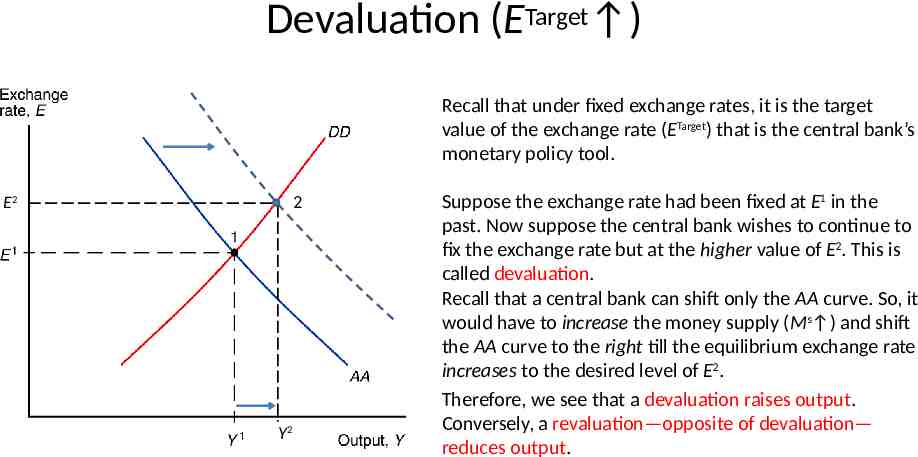
Devaluation (ETarget ) Recall that under fixed exchange rates, it is the target value of the exchange rate (ETarget) that is the central bank’s monetary policy tool. 2 E2 Y2 Suppose the exchange rate had been fixed at E1 in the past. Now suppose the central bank wishes to continue to fix the exchange rate but at the higher value of E2. This is called devaluation. Recall that a central bank can shift only the AA curve. So, it would have to increase the money supply (Ms ) and shift the AA curve to the right till the equilibrium exchange rate increases to the desired level of E2. Therefore, we see that a devaluation raises output. Conversely, a revaluation—opposite of devaluation— reduces output.

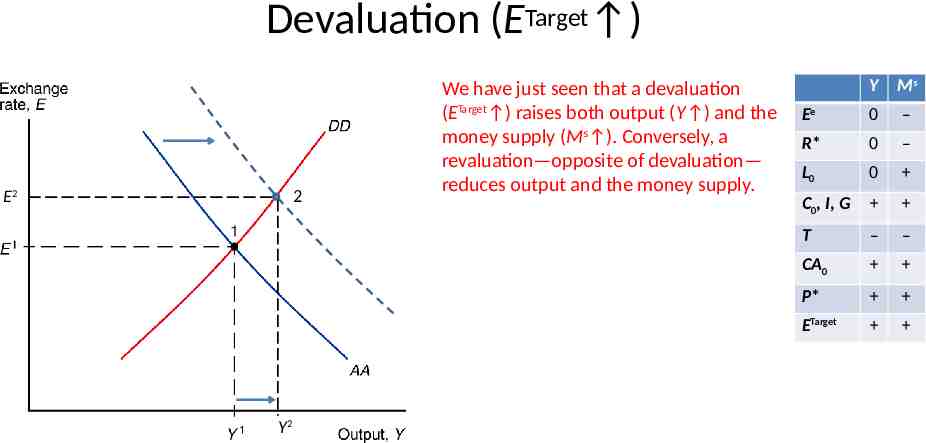
Devaluation (ETarget ) 2 E2 Y2 We have just seen that a devaluation (ETarget ) raises both output (Y ) and the money supply (Ms ). Conversely, a revaluation—opposite of devaluation— reduces output and the money supply. Y Ms Ee 0 – R* 0 – L0 0 C0, I, G T – – CA0 P* ETarget

Devaluation and Expectations The effects of a devaluation also depend on whether the new target value of the exchange rate (ETarget) is expected to continue for the foreseeable future If the new higher value of ETarget is expected to continue, then, logically, the expected future value of the exchange rate must also increase (E must imply Ee ) On the other hand, if the new value of ETarget is not expected to continue, then E would not imply Ee .

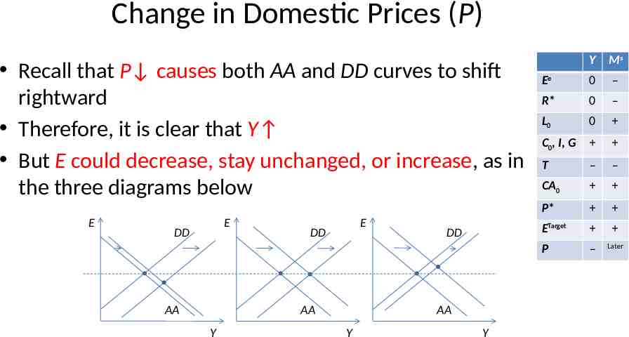
Change in Domestic Prices (P) Recall that P causes both AA and DD curves to shift rightward Therefore, it is clear that Y But E could decrease, stay unchanged, or increase, as in the three diagrams below E E DD AA E DD AA Y DD AA Y Y Y Ms Ee 0 – R* 0 – L0 0 C0, I, G T – – CA0 P* ETarget P – Later

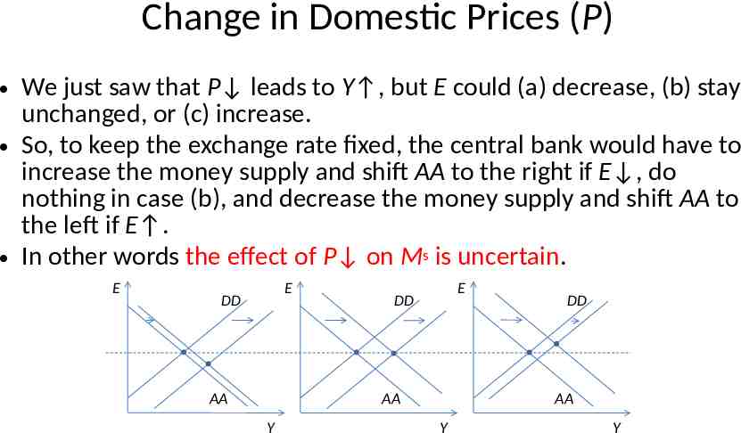
Change in Domestic Prices (P) We just saw that P leads to Y , but E could (a) decrease, (b) stay unchanged, or (c) increase. So, to keep the exchange rate fixed, the central bank would have to increase the money supply and shift AA to the right if E , do nothing in case (b), and decrease the money supply and shift AA to the left if E . In other words the effect of P on Ms is uncertain. E E DD AA E DD AA Y DD AA Y Y

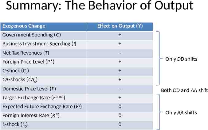
Summary: The Behavior of Output Exogenous Change Effect on Output (Y) Government Spending (G) Business Investment Spending (I) Net Tax Revenues (T) – Foreign Price Level (P*) C-shock (C0) CA-shocks (CA0) Domestic Price Level (P) – Target Exchange Rate (Etarget) Expected Future Exchange Rate (Ee) 0 Foreign Interest Rate (R*) 0 L-shock (L0) 0 Only DD shifts Both DD and AA shift Only AA shifts

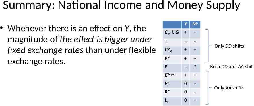
Summary: National Income and Money Supply Whenever there is an effect on Y, the magnitude of the effect is bigger under fixed exchange rates than under flexible exchange rates. Y Ms C0, I, G T – – CA0 P* P – ? ETarget Ee 0 – R* 0 – L0 0 Only DD shifts Both DD and AA shift Only AA shifts

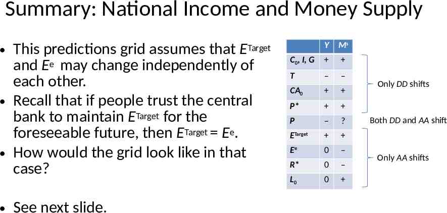
Summary: National Income and Money Supply This predictions grid assumes that E and Ee may change independently of each other. Recall that if people trust the central bank to maintain ETarget for the foreseeable future, then ETarget Ee. How would the grid look like in that case? Y Ms C0, I, G T – – CA0 P* P – ? ETarget Ee 0 – R* 0 – L0 0 Target See next slide. Only DD shifts Both DD and AA shift Only AA shifts

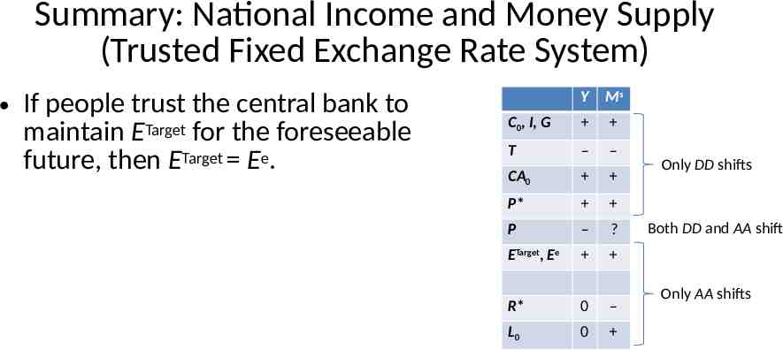
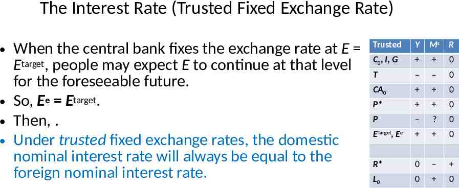
Summary: National Income and Money Supply (Trusted Fixed Exchange Rate System) If people trust the central bank to maintain ETarget for the foreseeable future, then ETarget Ee. Y Ms C0, I, G T – – CA0 P* P – ? ETarget, Ee R* 0 – L0 0 Only DD shifts Both DD and AA shift Only AA shifts

THE INTEREST RATE

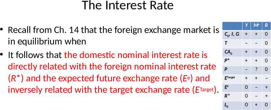
The Interest Rate Recall from Ch. 14 that the foreign exchange market is in equilibrium when It follows that the domestic nominal interest rate is directly related with the foreign nominal interest rate (R*) and the expected future exchange rate (Ee) and inversely related with the target exchange rate (ETarget). Y Ms R C0, I, G 0 T – – 0 CA0 0 P* 0 P – ? 0 ETarget – Ee 0 – R* 0 – L0 0 0

The Interest Rate (Trusted Fixed Exchange Rate) When the central bank fixes the exchange rate at E Etarget, people may expect E to continue at that level for the foreseeable future. So, Ee Etarget. Then, . Under trusted fixed exchange rates, the domestic nominal interest rate will always be equal to the foreign nominal interest rate. Trusted Y Ms R C0, I, G 0 T – – 0 CA0 0 P* 0 P – ? 0 ETarget, Ee 0 R* 0 – L0 0 0

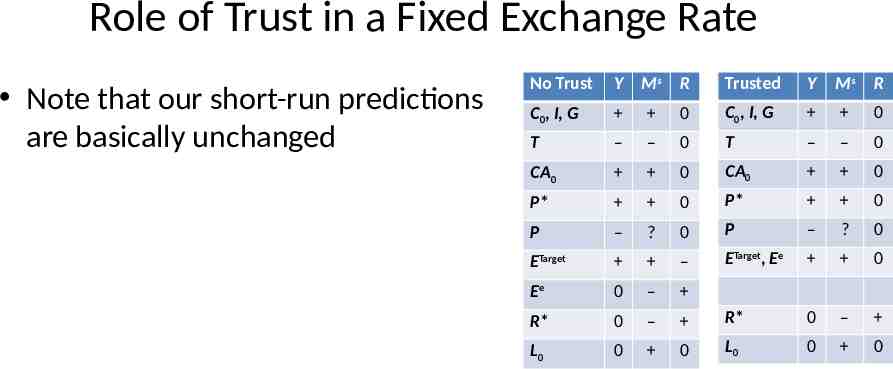
Role of Trust in a Fixed Exchange Rate Note that our short-run predictions are basically unchanged No Trust Y Ms R Trusted Y Ms R C0, I, G 0 C0, I, G 0 T – – 0 T – – 0 CA0 0 CA0 0 P* 0 P* 0 P – ? 0 P – ? 0 ETarget – ETarget, Ee 0 Ee 0 – R* 0 – R* 0 – L0 0 0 L0 0 0

THE CURRENT ACCOUNT

The Current Account Recall from Ch. 17 that there are two ways of expressing the domestic country’s net exports (or, current account): Method 1: Method 2:

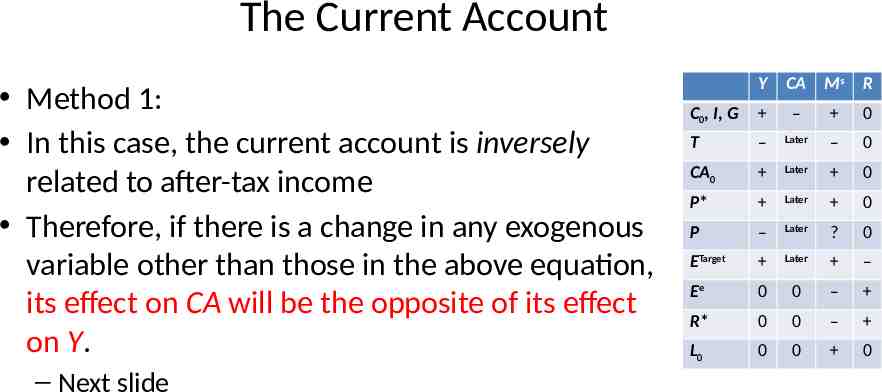
The Current Account Method 1: In this case, the current account is inversely related to after-tax income Therefore, if there is a change in any exogenous variable other than those in the above equation, its effect on CA will be the opposite of its effect on Y. – Next slide Y CA Ms R C0, I, G – 0 T – Later – 0 CA0 Later 0 P* Later 0 P – Later ? 0 ETarget Later – Ee 0 0 – R* 0 0 – L0 0 0 0

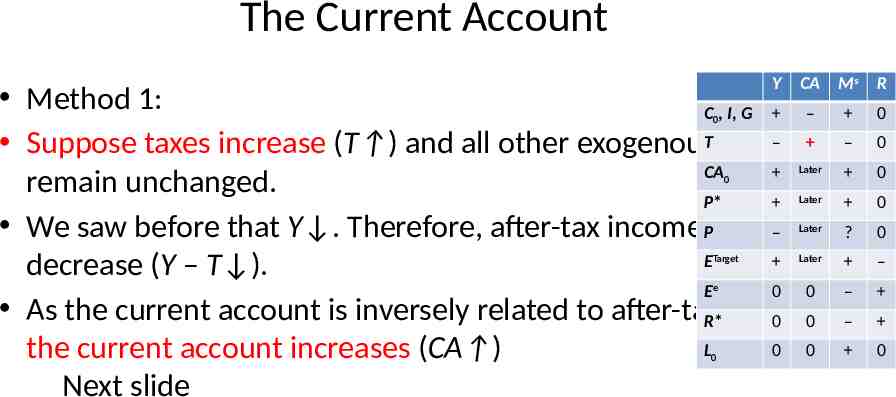
The Current Account Y CA Ms Method 1: C , I, G – – – Suppose taxes increase (T ) and all other exogenousT variables CA remain unchanged. P* We saw before that Y . Therefore, after-tax income Pmust– ? E decrease (Y – T ). E 0 0 – As the current account is inversely related to after-tax R* income, 0 0 – L 0 0 the current account increases (CA ) Next slide 0 0 Target e 0 R 0 0 Later 0 Later 0 Later 0 Later – 0

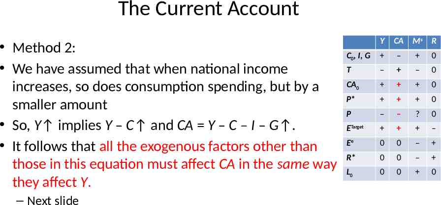
The Current Account Method 2: We have assumed that when national income increases, so does consumption spending, but by a smaller amount So, Y implies Y – C and CA Y – C – I – G . It follows that all the exogenous factors other than those in this equation must affect CA in the same way they affect Y. – Next slide Y CA Ms R C0, I, G – 0 T – – 0 CA0 0 P* 0 P – – ? 0 ETarget – Ee 0 0 – R* 0 0 – L0 0 0 0

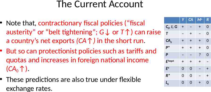
The Current Account Note that, contractionary fiscal policies (“fiscal austerity” or “belt tightening”; G or T ) can raise a country’s net exports (CA ) in the short run. But so can protectionist policies such as tariffs and quotas and increases in foreign national income (CA0 ). These predictions are also true under flexible exchange rates. Y CA Ms R C0, I, G – 0 T – – 0 CA0 0 P* 0 P – – ? 0 ETarget – Ee 0 0 – R* 0 0 – L0 0 0 0

REAL EXCHANGE RATE

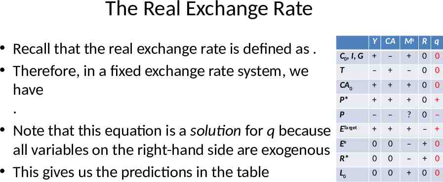
The Real Exchange Rate Recall that the real exchange rate is defined as . Therefore, in a fixed exchange rate system, we have . Note that this equation is a solution for q because all variables on the right-hand side are exogenous This gives us the predictions in the table Y CA Ms R q C0, I, G – 0 0 T – – 0 0 CA0 0 0 P* 0 P – – ? 0 – ETarget – Ee 0 0 – 0 R* 0 0 – 0 L0 0 0 0 0

COMPARING FLEXIBLE AND FIXED EXCHANGE RATE REGIMES

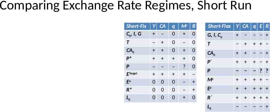
Comparing Exchange Rate Regimes, Short Run Short-Fix C0, I, G Y CA – q 0 Ms R 0 T CA0 – 0 0 – 0 0 P* P ETarget Ee R* L0 – 0 0 0 – 0 0 0 – 0 0 0 ? – – 0 0 – 0 Short-Flex Y CA q E R G, I, C0 T CA0 P* P ? ? Ms Ee R* L0

Comparing the Regimes As output (Y) and the current account (CA) are usually the two main topics, let us look at how the various exogenous variables affect Y and CA in the two exchange rate regimes

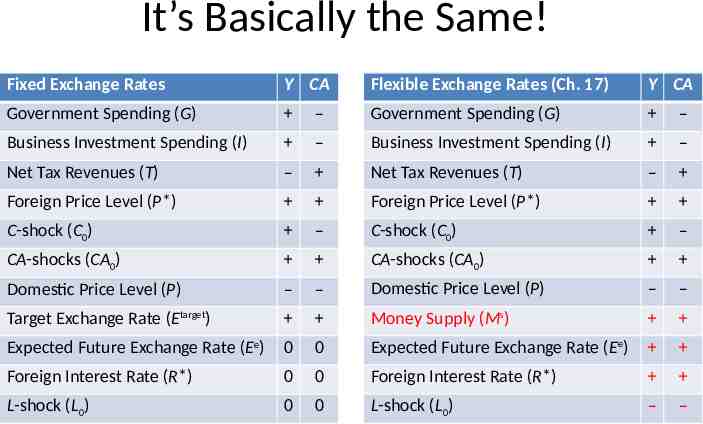
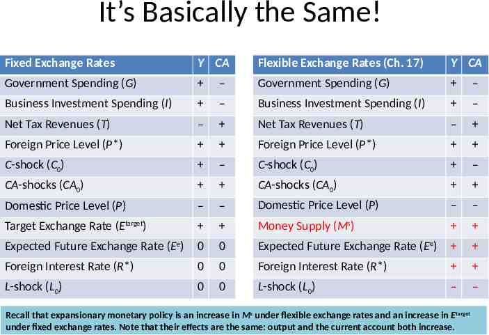
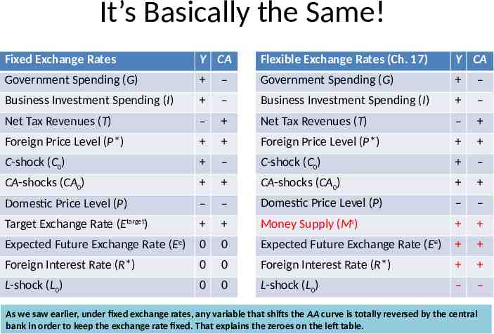
It’s Basically the Same! Fixed Exchange Rates Y CA Flexible Exchange Rates (Ch. 17) Y CA Government Spending (G) – Government Spending (G) – Business Investment Spending (I) – Business Investment Spending (I) – Net Tax Revenues (T) – Net Tax Revenues (T) – Foreign Price Level (P*) Foreign Price Level (P*) C-shock (C0) – C-shock (C0) – CA-shocks (CA0) CA-shocks (CA0) Domestic Price Level (P) – – Domestic Price Level (P) – – Target Exchange Rate (Etarget) Money Supply (Ms) Expected Future Exchange Rate (Ee) 0 0 Expected Future Exchange Rate (Ee) Foreign Interest Rate (R*) 0 0 Foreign Interest Rate (R*) L-shock (L0) 0 0 L-shock (L0) – –

BALANCE OF PAYMENTS CRISES

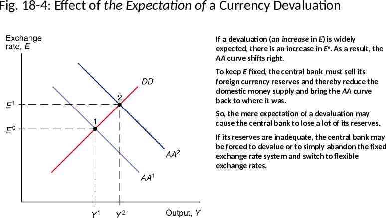
Fig. 18-4: Effect of the Expectation of a Currency Devaluation If a devaluation (an increase in E) is widely expected, there is an increase in Ee. As a result, the AA curve shifts right. To keep E fixed, the central bank must sell its foreign currency reserves and thereby reduce the domestic money supply and bring the AA curve back to where it was. So, the mere expectation of a devaluation may cause the central bank to lose a lot of its reserves. If its reserves are inadequate, the central bank may be forced to devalue or to simply abandon the fixed exchange rate system and switch to flexible exchange rates.

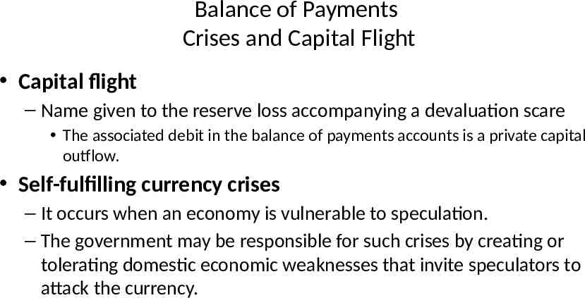
Balance of Payments Crises and Capital Flight Balance of payments crisis – It is a sharp fall in official foreign reserves sparked by a change in expectations about the future exchange rate.

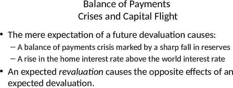
Balance of Payments Crises and Capital Flight The mere expectation of a future devaluation causes: – A balance of payments crisis marked by a sharp fall in reserves – A rise in the home interest rate above the world interest rate An expected revaluation causes the opposite effects of an expected devaluation.

Balance of Payments Crises and Capital Flight Capital flight – Name given to the reserve loss accompanying a devaluation scare The associated debit in the balance of payments accounts is a private capital outflow. Self-fulfilling currency crises – It occurs when an economy is vulnerable to speculation. – The government may be responsible for such crises by creating or tolerating domestic economic weaknesses that invite speculators to attack the currency.

THE LONG RUN UNDER FIXED EXCHANGE RATES

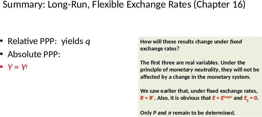
Summary: Long-Run, Flexible Exchange Rates (Chapter 16) Relative PPP: yields q Absolute PPP: Y Yf How will these results change under fixed exchange rates? The first three are real variables. Under the principle of monetary neutrality, they will not be affected by a change in the monetary system. We saw earlier that, under fixed exchange rates, R R*. Also, it is obvious that E Etarget and Eg 0. Only P and π remain to be determined.

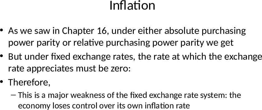
Inflation As we saw in Chapter 16, under either absolute purchasing power parity or relative purchasing power parity we get But under fixed exchange rates, the rate at which the exchange rate appreciates must be zero: Therefore, – This is a major weakness of the fixed exchange rate system: the economy loses control over its own inflation rate

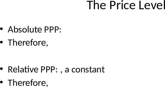
The Price Level Absolute PPP: Therefore, Relative PPP: , a constant Therefore,

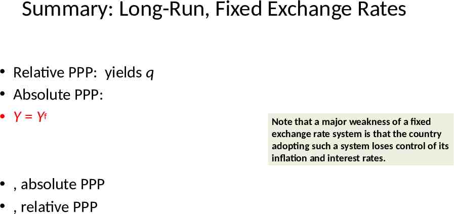
Summary: Long-Run, Fixed Exchange Rates Relative PPP: yields q Absolute PPP: Y Yf , absolute PPP , relative PPP Note that a major weakness of a fixed exchange rate system is that the country adopting such a system loses control of its inflation and interest rates.

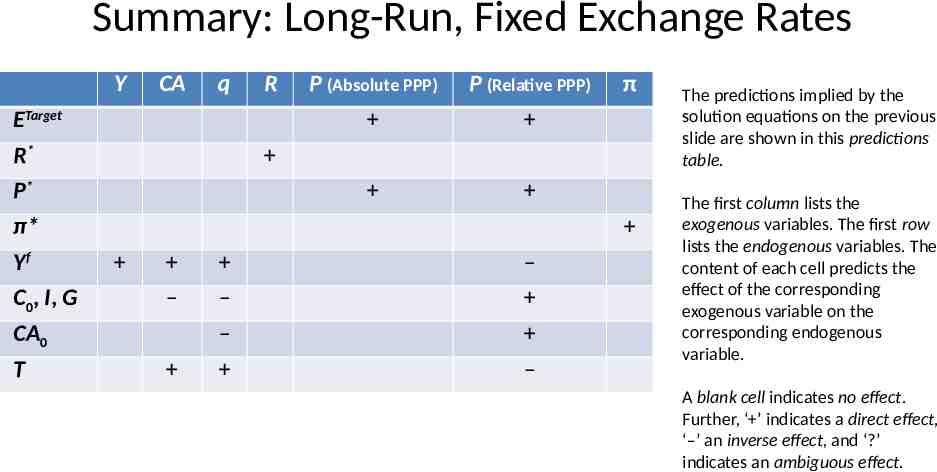
Summary: Long-Run, Fixed Exchange Rates Y ETarget R* P* π* Yf C0, I, G CA0 T CA q R P (Absolute PPP) P (Relative PPP) π – – – – – The predictions implied by the solution equations on the previous slide are shown in this predictions table. The first column lists the exogenous variables. The first row lists the endogenous variables. The content of each cell predicts the effect of the corresponding exogenous variable on the corresponding endogenous variable. A blank cell indicates no effect. Further, ‘ ’ indicates a direct effect, ‘–’ an inverse effect, and ‘?’ indicates an ambiguous effect.

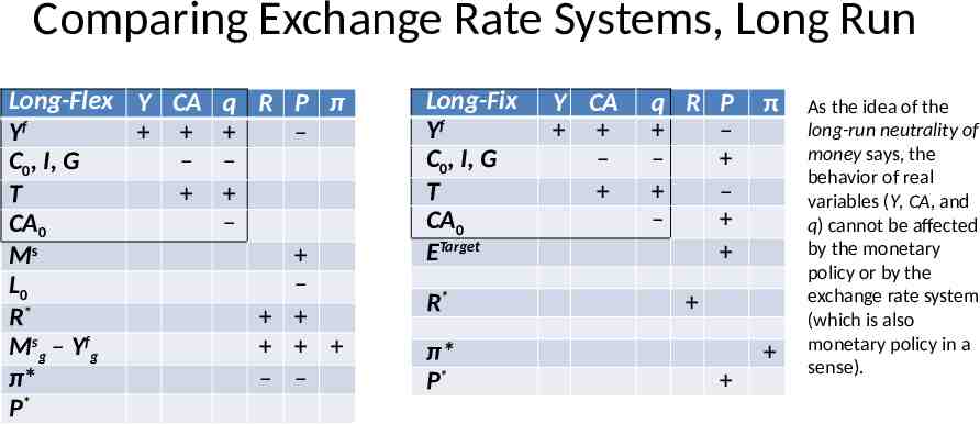
Comparing Exchange Rate Systems, Long Run Long-Flex Y CA q R P π Yf – – – C0, I, G T – CA0 Ms – L0 R* M s g – Y fg π* – – P* Long-Fix Yf C0, I, G T CA0 ETarget R* π* P* Y CA – q R P – – – – π As the idea of the long-run neutrality of money says, the behavior of real variables (Y, CA, and q) cannot be affected by the monetary policy or by the exchange rate system (which is also monetary policy in a sense).

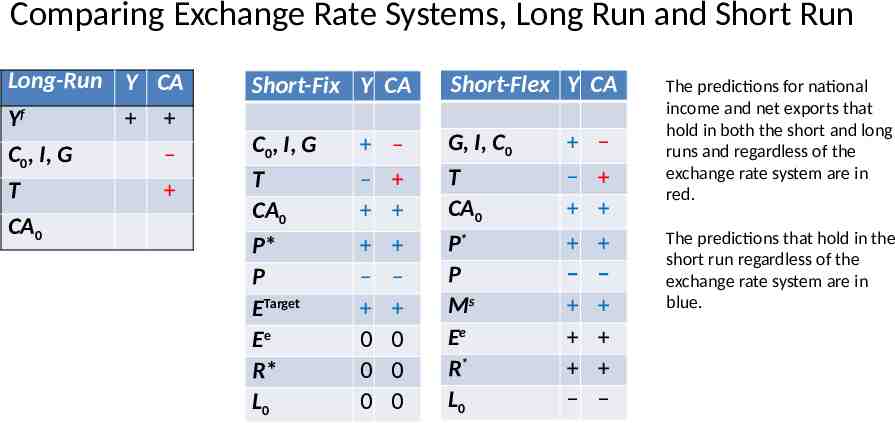
Comparing Exchange Rate Systems, Long Run and Short Run Long-Run Y CA Yf – C0, I, G T CA0 Short-Fix Y CA Short-Flex Y CA C0, I, G T CA0 P* P ETarget Ee R* L0 G, I, C0 T CA0 P* P Ms Ee R* L0 – – 0 0 0 – – 0 0 0 The predictions for national income and net exports that hold in both the short and long runs and regardless of the exchange rate system are in red. The predictions that hold in the short run regardless of the exchange rate system are in blue.

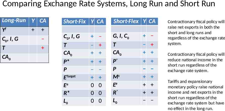
Comparing Exchange Rate Systems, Long Run and Short Run Long-Run Y CA Yf – C0, I, G T CA0 Short-Fix Y CA Short-Flex Y CA C0, I, G T CA0 P* P ETarget Ee R* L0 G, I, C0 T CA0 P* P Ms Ee R* L0 – – 0 0 0 – – 0 0 0 Contractionary fiscal policy will raise net exports in both the short and long runs and regardless of the exchange rate system. Contractionary fiscal policy will reduce national income in the short run regardless of the exchange rate system. Tariffs and expansionary monetary policy raise national income and net exports in the short run regardless of the exchange rate system but have no effect in the long run.

June 22, 2023

45 Less than a minute

Related Articles

Microsoft Azure Overview Ken Casada Technical Evangelist Microsoft

Choosing a Business Structure Before you start your

CMMI Overview Presented by: Bruce Boyd 28 January 2004 CMMI Overview

Electricity – Lesson 1 SP5a Develop and use mathematical models

ROYAUME DU MAROC Ministère de l’Equipement, du Transport et de la

Stepped Care Model for Pain Management Nabiha Gill, MD Staff