EE490 Signals and Systems Week 2 Laboratory Analysis of

EE490 Signals and Systems Week 2 Laboratory Analysis of System’s Response and Characteristic Roots (System’s Modes) Using MATLAB S. Stan Lan, Ph.D. Professor, College of Engineering and Information Sciences 1 7/8/24

OBJECTIVES – to be able to: Solve the system's first-order and high-order differential equations (obtain time domain response) using MATLAB. Plot the time domain response using MATLAB. Determine a system's stability by analyzing the system’s characteristic equations and the system’s characteristic roots. Determine a high-order system's stability by plotting its time domain response. 7/8/24 2

PROCEDURE Understand the illustrative examples. First order case High order case Execute the lab steps. Step 1: System’s Response Step 2:Calculating High-order Characteristic Roots and Plot Time Response 7/8/24 3

Illustrative Example: Obtain First Order System Solution Given To solve this first order differential equation using MATLAB, enter: y dsolve('Dy 5.5*y 1, y(0) -3') The answer is: y 2/11 - (35*exp(-(11*t)/2))/11 Therefore the solution is: 7/8/24 4

Illustrative Example: Plot First Order System Response Enter (you may adjust the time scale to obtain better view): t 6:.01:0; y 2/11 - (35*exp(-(11*t)/2))/11;plot(t,y), title('Time-domain Response of First-order System'); xlabel('Time'); ylabel('Timedomain Response'); grid on Therefore the plot is: 14 0 Time-domain Response of First-order System x 10 -1 Time-domain Response -2 -3 -4 -5 -6 -7 -6 -5 -4 -3 Time -2 -1 0 7/8/24 5

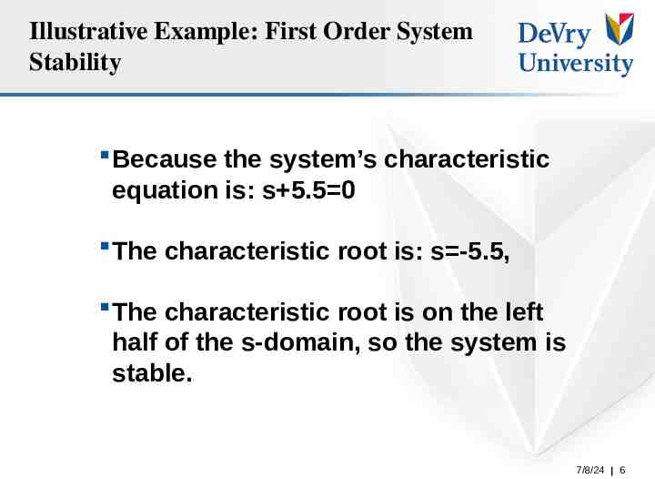
Illustrative Example: First Order System Stability Because the system’s characteristic equation is: s 5.5 0 The characteristic root is: s -5.5, The characteristic root is on the left half of the s-domain, so the system is stable. 7/8/24 6

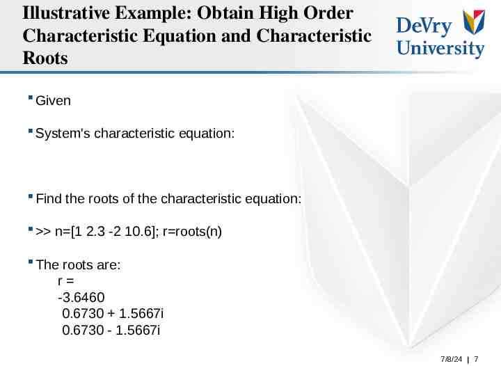
Illustrative Example: Obtain High Order Characteristic Equation and Characteristic Roots Given System's characteristic equation: Find the roots of the characteristic equation: n [1 2.3 -2 10.6]; r roots(n) The roots are: r -3.6460 0.6730 1.5667i 0.6730 - 1.5667i 7/8/24 7

Illustrative Example: High Order System Stability What are your conclusions about the stability? Elaborate on the stability criteria to theoretically support your conclusion. 7/8/24 8

Illustrative Example: Solve for Time Domain Solution for the High Order System To solve the given high order differential equation using MATLAB, enter (assume all initial conditions are zero): y dsolve('D3y 2.3*D2y-2*Dy 10.6*y 1, D2y(0) 0, Dy(0) 0, y(0) 0') The obtained time-domain solution is: y (10*exp(-t*(1129/(900*(175967/27000 (135000 (1/2)*5467651 (1/2))/135000) (1/3)) 1274641)) 5/53 It’s an extremely long and complicated answer. To solve for it by hand is humanly impossible! 7/8/24 9

Illustrative Example: To Plot the High Order System’s Time Response t 0:.01:30; y (10.*exp(-t.*(1129./(900.*(175967./27000 - 1274641)) 5./53; plot(t,y); title('Time-domain Response of Highorder System'); xlabel('Time'); ylabel('Time-domain Response'); grid on Please see details in the Lab Instructions. 7 5 Time-domain Response of High-order System x 10 T im e-dom ain R es pons e 4 3 2 1 0 -1 -2 0 5 10 15 Time 20 25 30 7/8/24 10

Q&A Questions? E-mail: [email protected] Voicemail: 630-515-7726 7/8/24 11