EE 313 Linear Systems and Signals Fall 2021 Transfer Functions Prof.

EE 313 Linear Systems and Signals Fall 2021 Transfer Functions Prof. Brian L. Evans Dept. of Electrical and Computer Engineering The University of Texas at Austin Textbook: McClellan, Schafer & Yoder, Signal Processing First, 2003 Lecture 18 http://www.ece.utexas.edu/ bevans/courses/signals

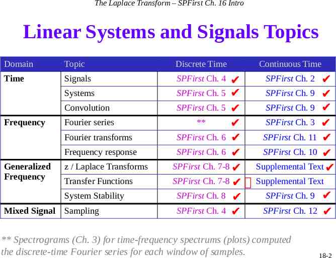
The Laplace Transform – SPFirst Ch. 16 Intro Linear Systems and Signals Topics Domain Topic Time Signals Systems Convolution Frequency Fourier series Fourier transforms Frequency response Generalized Frequency z / Laplace Transforms Transfer Functions System Stability Mixed Signal Sampling Discrete Time SPFirst Ch. 5 SPFirst Ch. 5 ** SPFirst Ch. 6 SPFirst Ch. 6 SPFirst Ch. 7-8 SPFirst Ch. 7-8 SPFirst Ch. 8 SPFirst Ch. 4 SPFirst Ch. 4 Continuous Time SPFirst Ch. 9 SPFirst Ch. 9 SPFirst Ch. 3 SPFirst Ch. 11 SPFirst Ch. 10 Supplemental Text SPFirst Ch. 2 Supplemental Text SPFirst Ch. 9 SPFirst Ch. 12 ** Spectrograms (Ch. 3) for time-frequency spectrums (plots) computed the discrete-time Fourier series for each window of samples. 18-2

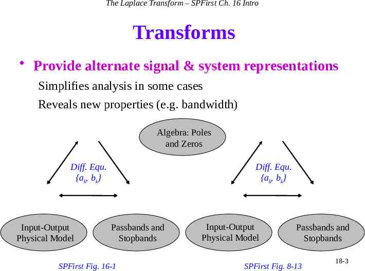
The Laplace Transform – SPFirst Ch. 16 Intro Transforms Provide alternate signal & system representations Simplifies analysis in some cases Reveals new properties (e.g. bandwidth) Algebra: Poles and Zeros Diff. Equ. {ak, bk} Input-Output Physical Model Diff. Equ. {ak, bk} Passbands and Stopbands SPFirst Fig. 16-1 Input-Output Physical Model Passbands and Stopbands SPFirst Fig. 8-13 18-3

Transfer Function Laplace transform of impulse response h(t) of linear time-invariant (LTI) system Convolution in time property: x(t) y(t) w(t) h1(t) X(s) W(s) W(s) H1(s) X(s) h2(t) Y(s) H2(s) W(s) H2(s) H1(s) X(s) y(t) x(t) X(s) See lecture slide 10-8 for discrete-time analogy Y(s) h(t) H(s) H2(s) H1(s) H1(s) H2(s) Y(s) 18-4

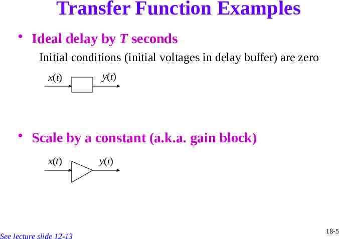
Transfer Function Examples Ideal delay by T seconds Initial conditions (initial voltages in delay buffer) are zero x(t) y(t) Scale by a constant (a.k.a. gain block) x(t) See lecture slide 12-13 y(t) 18-5

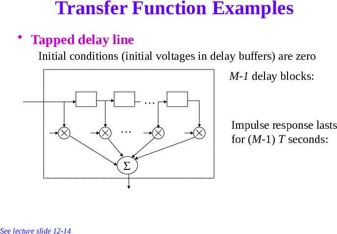
Transfer Function Examples Tapped delay line Initial conditions (initial voltages in delay buffers) are zero M-1 delay blocks: S See lecture slide 12-14 Impulse response lasts for (M-1) T seconds:

Transfer Function Examples Ideal integrator with y(0-) 0 for LTI to hold x(t) y(t) x(t) 0 See lecture slide 12-12 Ideal differentiator with x(0-) 0 for LTI to hold y(t) 0 18-7

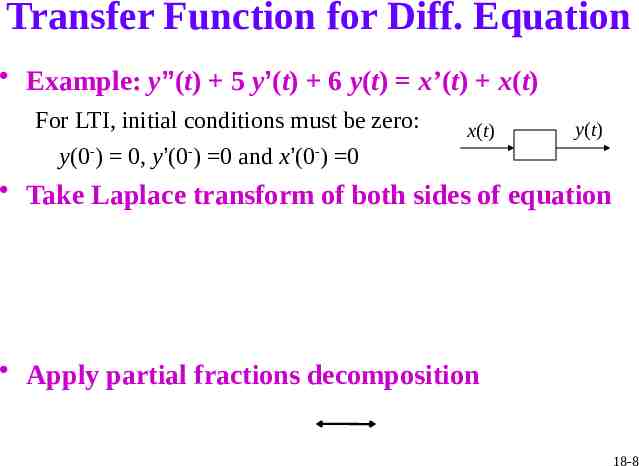
Transfer Function for Diff. Equation Example: y”(t) 5 y’(t) 6 y(t) x’(t) x(t) For LTI, initial conditions must be zero: y(0-) 0, y’(0-) 0 and x’(0-) 0 x(t) y(t) Take Laplace transform of both sides of equation Apply partial fractions decomposition 18-8

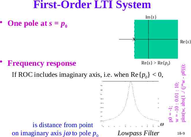
First-Order LTI System Im{s} One pole at s p0 X Re{s} Re{p0} If ROC includes imaginary axis, i.e. when Re{p0} 0, is distance from point on imaginary axis jw to pole p0 w Lowpass Filter p0 -1; w -10 : 0.01 : 10; plot(w, abs(1 ./ (j*w - p0))); Frequency response Re{s} 18-9

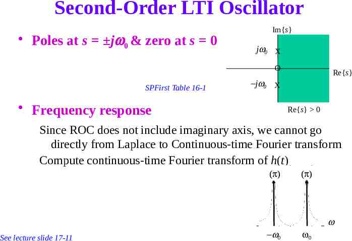
Second-Order LTI Oscillator Poles at s jw0 & zero at s 0 Im{s} jw0 X O SPFirst Table 16-1 Re{s} -j w 0 X Frequency response Re{s} 0 Since ROC does not include imaginary axis, we cannot go directly from Laplace to Continuous-time Fourier transform Compute continuous-time Fourier transform of h(t) (p) (p) w See lecture slide 17-11 -w0 w0

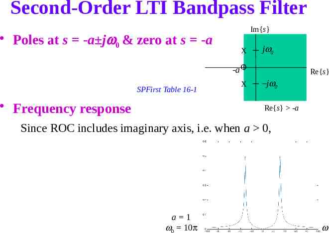
Second-Order LTI Bandpass Filter Poles at s -a jw0 & zero at s -a Im{s} X jw 0 -a O SPFirst Table 16-1 Frequency response X Re{s} - jw 0 Re{s} -a Since ROC includes imaginary axis, i.e. when a 0, a 1 w0 10p w

LTI Systems in Cascade and Parallel Cascade X(s) H1(s) H2(s) Y(s) H2(s) X(s) H1(s) Y(s) W(s) H1(s) X(s) Y(s) H2(s)W(s) Y(s) H1(s) H2(s) X(s) Y(s)/X(s) H1(s)H2(s) H(s) One can switch order of the cascade of two LTI systems if both LTI systems represent amplitudes in exact precision Parallel combination Use partial fractions to decompose a transfer function H(s) G1(s) G2(s) Y(s) G1(s)X(s) G2(s)X(s) Y(s)/X(s) G1(s) G2(s) G1(s) X(s) G2(s) Y(s) X(s) G1(s) G2(s) Y(s) Advantages of parallel vs. cascade combination? 18-12

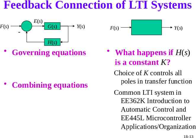
Feedback Connection of LTI Systems F(s) - E(s) G(s) Y(s) F(s) Y(s) H(s) Governing equations Combining equations What happens if H(s) is a constant K? Choice of K controls all poles in transfer function Common LTI system in EE362K Introduction to Automatic Control and EE445L Microcontroller Applications/Organization 18-13

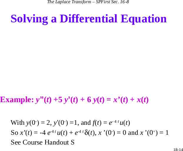
The Laplace Transform – SPFirst Sec. 16-8 Solving a Differential Equation Example: y”(t) 5 y’(t) 6 y(t) x’(t) x(t) With y(0-) 2, y’(0-) 1, and f(t) e- 4 t u(t) So x’(t) -4 e-4 t u(t) e-4 t d(t), x ’(0-) 0 and x ’(0 ) 1 See Course Handout S 18-14