Earthquakes recorded in the landscape: Using digital topography to

Earthquakes recorded in the landscape: Using digital topography to investigate earthquake faulting Christopher Crosby GEON / Arizona State University SDSC TeacherTech Seminar Wednesday, February 27, 2008, 4:30pm- 6:30pm

Outline Introduction to earthquakes, plate tectonic deformation and the San Andreas fault – Exercise: GPS observations of deformation around the San Andreas Introduction to digital topography, earthquake faulting and long and short-term fault deformation – Exercise: Google Earth and digital topography to document offset features and investigate earthquake behavior

Introduction I Goal: Develop a basic understanding of plate tectonics-driven deformation. Questions: – What tools do researchers use to study tectonic motion? – How is plate tectonic motion distributed across California – where do you expect to have EQs? – Do our observations of plate tectonics agree with where we see earthquakes?

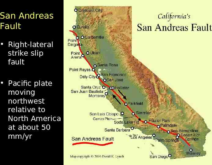
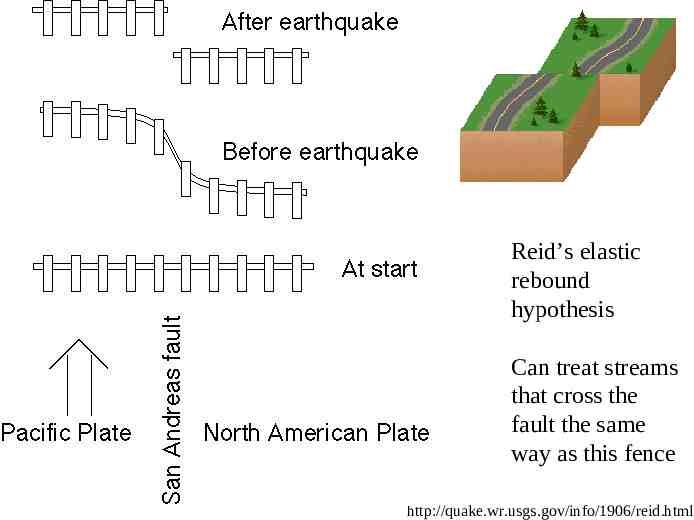
San Andreas Fault Right-lateral strike slip fault Pacific plate moving northwest relative to North America at about 50 mm/yr

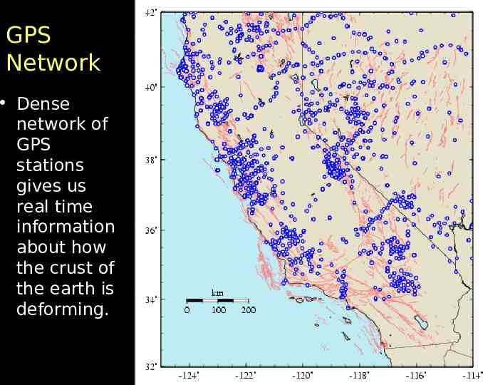
Plate boundary deformation Is all 50 mm/yr of Pacific/North American plate motion on the SAF? If not, how is this deformation distributed? Can use GPS to answer this question

GPS Network Dense network of GPS stations gives us real time information about how the crust of the earth is deforming.

Exercise 1 pdf

Reverse (or Thrust) faults are found where the crust is in compression. GPS velocity transect parallel to the SAF shows a decline in plate motion to the north how is the greater deformation rate to the south accommodated?

Introduction II Goal: Illustrate the linkage between plate tectonics and evidence for earthquakes in the landscape. – How can high-resolution topography help us study earthquakes? – What do fault related landforms tell us about long-term fault activity? What do the landforms tell us about short-term fault activity? – Introduction to the concepts of slip rate, slip per event, recurrence and characteristic EQs

1906 earthquake surface rupture. 8’ fence offset above http://mnw.eas.slu.edu/Earthquake C enter/1906EQ/1906thumb.html And http://quake.wr.usgs.gov/info/1906/i mages/fenceoffset big.html

Reid’s elastic rebound hypothesis Can treat streams that cross the fault the same way as this fence http://quake.wr.usgs.gov/info/1906/reid.html

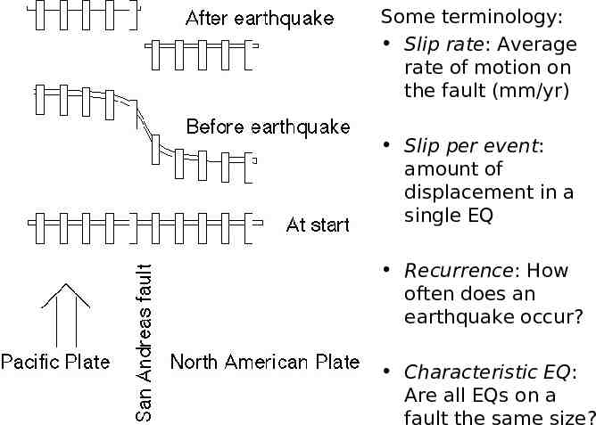
Some terminology: Slip rate: Average rate of motion on the fault (mm/yr) Slip per event: amount of displacement in a single EQ Recurrence: How often does an earthquake occur? Characteristic EQ: Are all EQs on a fault the same size?

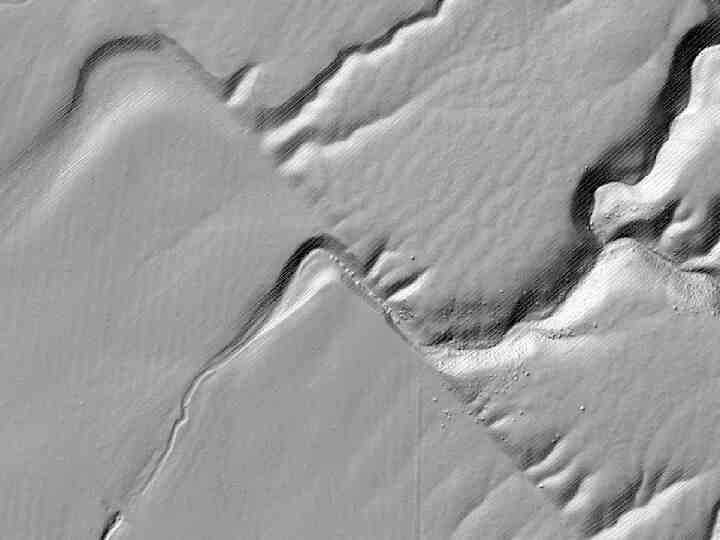
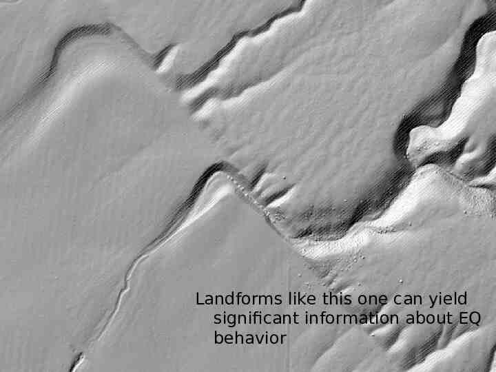
Landforms like this one can yield significant information about EQ behavior

Wallace Creek development. Sieh and Wallace, 1987

LiDAR (LIght Detection And Ranging) a.k.a ALSM (Airborne Laser Swath Mapping) Airborne pulsed laser scanning system differential GPS inertial measurement unit (IMU) 30,000 points/second Ground sampled multiple points/sq. meter 15 cm vertical accuracy http://coastal.er.usgs.gov/hurricanes/mappingchange/ 300 - 500 per sq. km acquisition cost

LiDAR “point cloud” x,y,z attributes

Exercise 2 pdf http://lidar.asu.edu/TeacherTech08.html