DTC Quantitative Methods Bivariate Analysis: Cross-tabulations

DTC Quantitative Methods Bivariate Analysis: Cross-tabulations and Chi-square Thursday 23rd February 2012

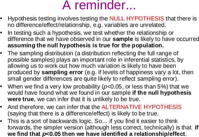
A reminder. Hypothesis testing involves testing the NULL HYPOTHESIS that there is no difference/effect/relationship, e.g. variables are unrelated. In testing such a hypothesis, we test whether the relationship or difference that we have observed in our sample is likely to have occurred assuming the null hypothesis is true for the population. The sampling distribution (a distribution reflecting the full range of possible samples) plays an important role in inferential statistics, by allowing us to work out how much variation is likely to have been produced by sampling error (e.g. if levels of happiness vary a lot, then small gender differences are quite likely to reflect sampling error). When we find a very low probability (p 0.05, or less than 5%) that we would have found what we found in our sample if the null hypothesis were true, we can infer that it is unlikely to be true. And therefore, we can infer that the ALTERNATIVE HYPOTHESIS (saying that there is a difference/effect) is likely to be true. This is a sort of backwards logic. So if you find it easier to think forwards, the simpler version (although less correct, technically) is that if we find that p 0.05 then we have identified a relationship/effect.

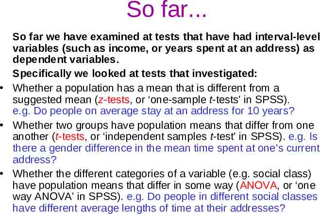
So far. So far we have examined at tests that have had interval-level variables (such as income, or years spent at an address) as dependent variables. Specifically we looked at tests that investigated: Whether a population has a mean that is different from a suggested mean (z-tests, or ‘one-sample t-tests’ in SPSS). e.g. Do people on average stay at an address for 10 years? Whether two groups have population means that differ from one another (t-tests, or ‘independent samples t-test’ in SPSS). e.g. Is there a gender difference in the mean time spent at one’s current address? Whether the different categories of a variable (e.g. social class) have population means that differ in some way (ANOVA, or ‘one way ANOVA’ in SPSS). e.g. Do people in different social classes have different average lengths of time at their addresses?

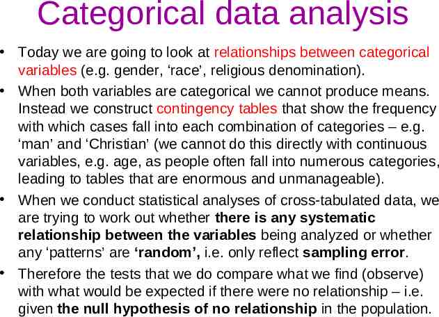
Categorical data analysis Today we are going to look at relationships between categorical variables (e.g. gender, ‘race’, religious denomination). When both variables are categorical we cannot produce means. Instead we construct contingency tables that show the frequency with which cases fall into each combination of categories – e.g. ‘man’ and ‘Christian’ (we cannot do this directly with continuous variables, e.g. age, as people often fall into numerous categories, leading to tables that are enormous and unmanageable). When we conduct statistical analyses of cross-tabulated data, we are trying to work out whether there is any systematic relationship between the variables being analyzed or whether any ‘patterns’ are ‘random’, i.e. only reflect sampling error. Therefore the tests that we do compare what we find (observe) with what would be expected if there were no relationship – i.e. given the null hypothesis of no relationship in the population.

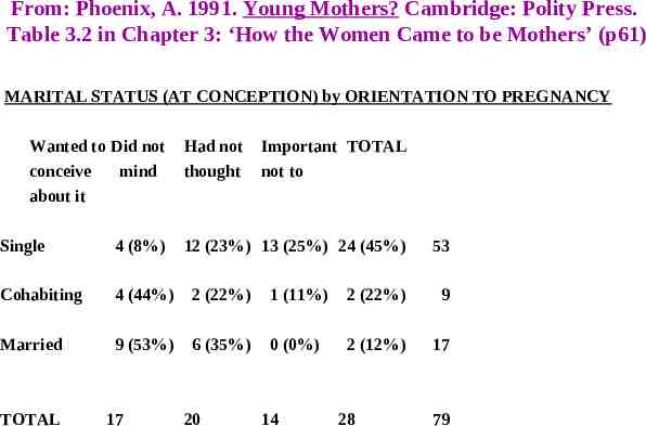
From: Phoenix, A. 1991. Young Mothers? Cambridge: Polity Press. Table 3.2 in Chapter 3: ‘How the Women Came to be Mothers’ (p61) MARITAL STATUS (AT CONCEPTION) by ORIENTATION TO PREGNANCY Wanted to Did not conceive mind about it Had not thought Important TOTAL not to Single 4 (8%) Cohabiting 4 (44%) 2 (22%) 1 (11%) 2 (22%) 9 Married 9 (53%) 6 (35%) 0 (0%) 2 (12%) 17 TOTAL 17 12 (23%) 13 (25%) 24 (45%) 20 14 28 53 79

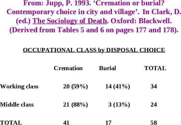
From: Jupp, P. 1993. ‘Cremation or burial? Contemporary choice in city and village’. In Clark, D. (ed.) The Sociology of Death. Oxford: Blackwell. (Derived from Tables 5 and 6 on pages 177 and 178). OCCUPATIONAL CLASS by DISPOSAL CHOICE Cremation Burial TOTAL Working class 20 (59%) 14 (41%) 34 Middle class 21 (88%) 3 (13%) 24 TOTAL 41 17 58

What can be learned from these cross-tabulations? Do you think that the patterns in the MARITAL STATUS by ORIENTATION TO PREGNANCY and OCCUPATIONAL CLASS by DISPOSAL CHOICE cross-tabulations provide sufficient evidence to conclude that relationships exist? Where can the relationship, if any, be found in the MARITAL STATUS (AT CONCEPTION) by ORIENTATION TO PREGNANCY cross-tabulation?

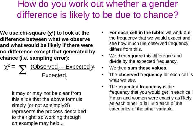
How do you work out whether a gender difference is likely to be due to chance? We use chi-square ( 2) to look at the difference between what we observe and what would be likely if there were no difference except that generated by chance (i.e. sampling error): 2 (Observedij – Expectedij)2 Expectedij It may or may not be clear from this slide that the above formula simply (or not so simply?!) represents the process described to the right, so working through an example may help. For each cell in the table: we work out the frequency that we would expect and see how much the observed frequency differs from this. We then square this difference and divide by the expected frequency. We then sum these values. The observed frequency for each cell is what we see. The expected frequency is the frequency that you would get in each cell if men and women were exactly as likely as each other to fall into each of the categories of the other variable.

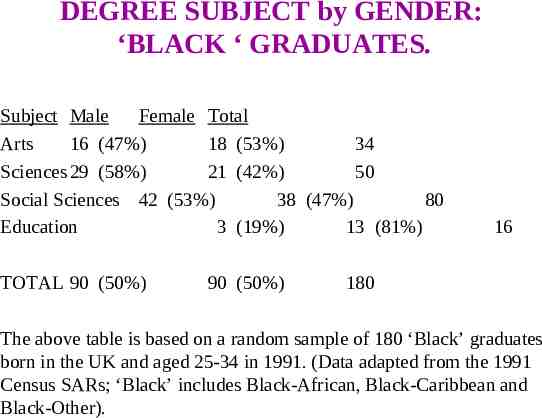
DEGREE SUBJECT by GENDER: ‘BLACK ‘ GRADUATES. Subject Male Female Total Arts 16 (47%) 18 (53%) 34 Sciences 29 (58%) 21 (42%) 50 Social Sciences 42 (53%) 38 (47%) 80 Education 3 (19%) 13 (81%) TOTAL 90 (50%) 90 (50%) 16 180 The above table is based on a random sample of 180 ‘Black’ graduates born in the UK and aged 25-34 in 1991. (Data adapted from the 1991 Census SARs; ‘Black’ includes Black-African, Black-Caribbean and Black-Other).

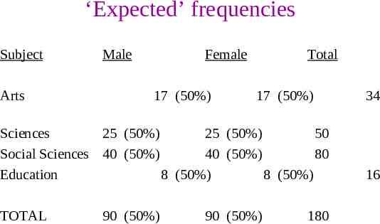
‘Expected’ frequencies Subject Arts Male Female 17 (50%) Total 17 (50%) Sciences 25 (50%) 25 (50%) 50 Social Sciences 40 (50%) 40 (50%) 80 Education 8 (50%) 8 (50%) TOTAL 90 (50%) 90 (50%) 180 34 16

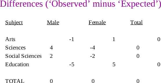
Differences (‘Observed’ minus ‘Expected’) Subject Male Arts Sciences Social Sciences Education 4 2 TOTAL 0 Female -1 Total 1 -4 -2 -5 0 0 0 5 0 0 0

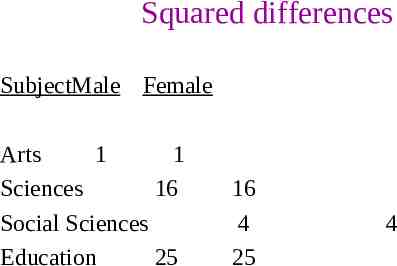
Squared differences SubjectMale Female Arts 1 1 Sciences 16 Social Sciences Education 25 16 4 25 4

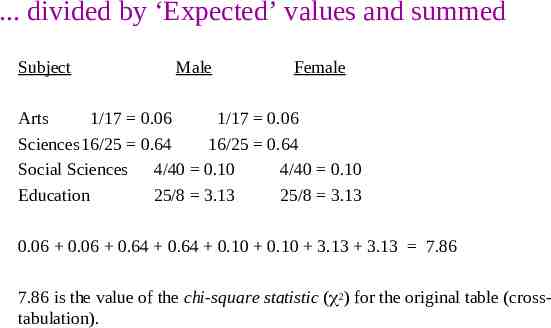
. divided by ‘Expected’ values and summed Subject Male Female Arts 1/17 0.06 1/17 0.06 Sciences16/25 0.64 16/25 0.64 Social Sciences 4/40 0.10 4/40 0.10 Education 25/8 3.13 25/8 3.13 0.06 0.06 0.64 0.64 0.10 0.10 3.13 3.13 7.86 7.86 is the value of the chi-square statistic ( 2) for the original table (crosstabulation).

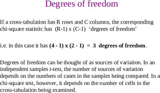
Degrees of freedom If a cross-tabulation has R rows and C columns, the corresponding chi-square statistic has (R-1) x (C-1) ‘degrees of freedom’ i.e. in this case it has (4 - 1) x (2 - 1) 3 degrees of freedom. Degrees of freedom can be thought of as sources of variation. In an independent samples t-test, the number of sources of variation depends on the numbers of cases in the samples being compared. In a chi-square test, however, it depends on the number of cells in the cross-tabulation being examined.

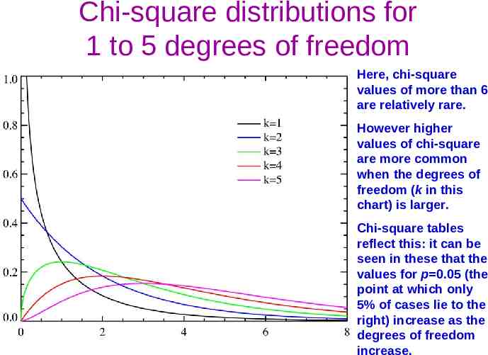
Chi-square distributions for 1 to 5 degrees of freedom Here, chi-square values of more than 6 are relatively rare. However higher values of chi-square are more common when the degrees of freedom (k in this chart) is larger. Chi-square tables reflect this: it can be seen in these that the values for p 0.05 (the point at which only 5% of cases lie to the right) increase as the degrees of freedom increase.

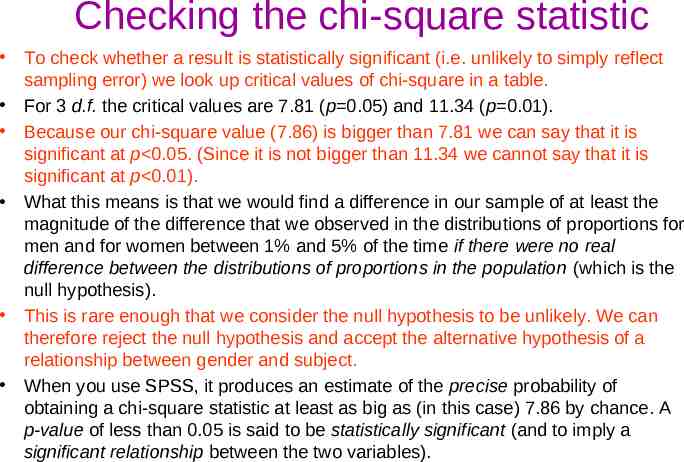
Checking the chi-square statistic To check whether a result is statistically significant (i.e. unlikely to simply reflect sampling error) we look up critical values of chi-square in a table. For 3 d.f. the critical values are 7.81 (p 0.05) and 11.34 (p 0.01). Because our chi-square value (7.86) is bigger than 7.81 we can say that it is significant at p 0.05. (Since it is not bigger than 11.34 we cannot say that it is significant at p 0.01). What this means is that we would find a difference in our sample of at least the magnitude of the difference that we observed in the distributions of proportions for men and for women between 1% and 5% of the time if there were no real difference between the distributions of proportions in the population (which is the null hypothesis). This is rare enough that we consider the null hypothesis to be unlikely. We can therefore reject the null hypothesis and accept the alternative hypothesis of a relationship between gender and subject. When you use SPSS, it produces an estimate of the precise probability of obtaining a chi-square statistic at least as big as (in this case) 7.86 by chance. A p-value of less than 0.05 is said to be statistically significant (and to imply a significant relationship between the two variables).

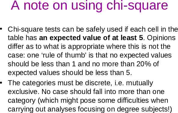
A note on using chi-square Chi-square tests can be safely used if each cell in the table has an expected value of at least 5. Opinions differ as to what is appropriate where this is not the case: one ‘rule of thumb’ is that no expected values should be less than 1 and no more than 20% of expected values should be less than 5. The categories must be discrete, i.e. mutually exclusive. No case should fall into more than one category (which might pose some difficulties when carrying out analyses focusing on degree subjects!)

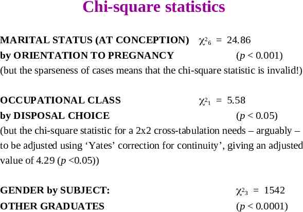
Chi-square statistics MARITAL STATUS (AT CONCEPTION) 26 24.86 by ORIENTATION TO PREGNANCY (p 0.001) (but the sparseness of cases means that the chi-square statistic is invalid!) OCCUPATIONAL CLASS 21 5.58 by DISPOSAL CHOICE (p 0.05) (but the chi-square statistic for a 2x2 cross-tabulation needs – arguably – to be adjusted using ‘Yates’ correction for continuity’, giving an adjusted value of 4.29 (p 0.05)) GENDER by SUBJECT: 23 1542 OTHER GRADUATES (p 0.0001)

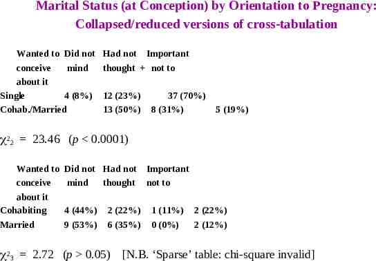
Marital Status (at Conception) by Orientation to Pregnancy: Collapsed/reduced versions of cross-tabulation Wanted to Did not conceive mind about it Single 4 (8%) Cohab./Married Had not Important thought not to 12 (23%) 13 (50%) 37 (70%) 8 (31%) 5 (19%) 22 23.46 (p 0.0001) Wanted to conceive about it Cohabiting Married Did not Had not mind thought 4 (44%) 9 (53%) 2 (22%) 6 (35%) Important not to 1 (11%) 0 (0%) 2 (22%) 2 (12%) 23 2.72 (p 0.05) [N.B. ‘Sparse’ table: chi-square invalid]

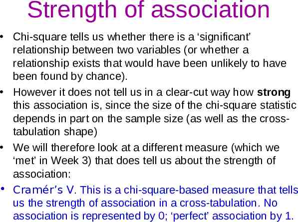
Strength of association Chi-square tells us whether there is a ‘significant’ relationship between two variables (or whether a relationship exists that would have been unlikely to have been found by chance). However it does not tell us in a clear-cut way how strong this association is, since the size of the chi-square statistic depends in part on the sample size (as well as the crosstabulation shape) We will therefore look at a different measure (which we ‘met’ in Week 3) that does tell us about the strength of association: Cramér’s V. This is a chi-square-based measure that tells us the strength of association in a cross-tabulation. No association is represented by 0; ‘perfect’ association by 1.

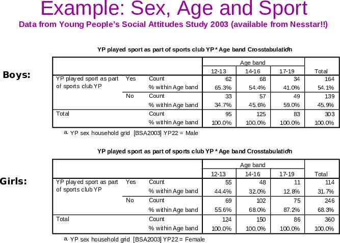
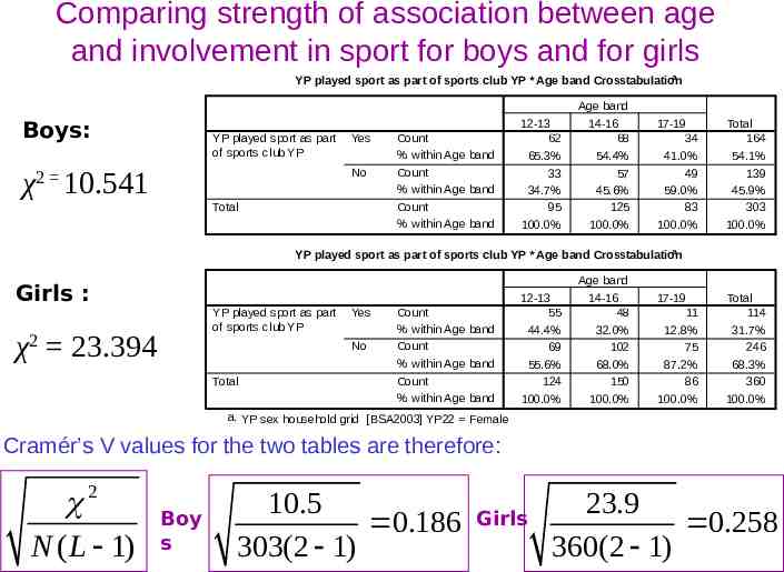
Example: Sex, Age and Sport Data from Young People’s Social Attitudes Study 2003 (available from Nesstar!!) a YP played sport as part of sports club YP * Age band Crosstabulation Boys: YP played sport as part of sports club YP Yes No Total Count % within Age band Count % within Age band Count % within Age band 12-13 62 65.3% 33 34.7% 95 100.0% Age band 14-16 68 54.4% 57 45.6% 125 100.0% 17-19 34 41.0% 49 59.0% 83 100.0% Total 164 54.1% 139 45.9% 303 100.0% a. YP sex household grid [BSA2003] YP22 Male a YP played sport as part of sports club YP * Age band Crosstabulation Girls: YP played sport as part of sports club YP Yes No Total Count % within Age band Count % within Age band Count % within Age band a. YP sex household grid [BSA2003] YP22 Female 12-13 55 44.4% 69 55.6% 124 100.0% Age band 14-16 48 32.0% 102 68.0% 150 100.0% 17-19 11 12.8% 75 87.2% 86 100.0% Total 114 31.7% 246 68.3% 360 100.0%

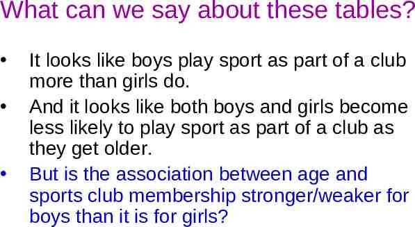
What can we say about these tables? It looks like boys play sport as part of a club more than girls do. And it looks like both boys and girls become less likely to play sport as part of a club as they get older. But is the association between age and sports club membership stronger/weaker for boys than it is for girls?

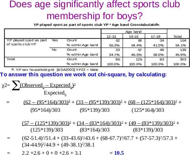
Does age significantly affect sports club membership for boys? a YP played sport as part of sports club YP * Age band Crosstabulation YP played sport as part of sports club YP Yes No Total Count % within Age band Count % within Age band Count % within Age band 12-13 62 65.3% 33 34.7% 95 100.0% Age band 14-16 68 54.4% 57 45.6% 125 100.0% 17-19 34 41.0% 49 59.0% 83 100.0% Total 164 54.1% 139 45.9% 303 100.0% a. YP sex household grid [BSA2003] YP22 Male To answer this question we work out chi-square, by calculating: χ2 (Observedij – Expectedij)2 Expectedij (62 – (95*164)/303)2 (33 – (95*139)/303)2 (68 – (125*164)/303)2 (95*164)/303 (95*139)/303 (125*164)/303 (57 – (125*139)/303)2 (34 – (83*164)/303)2 (49 – (83*139)/303)2 (125*139)/303 (83*164)/303 (83*139)/303 (62-51.4)2/51.4 (33-43.6)2/43.6 (68-67.7)2/67.7 (57-57.3)2/57.3 (34-44.9)2/44.9 (49-38.1)2/38.1 2.2 2.6 0 0 2.6 3.1 10.5

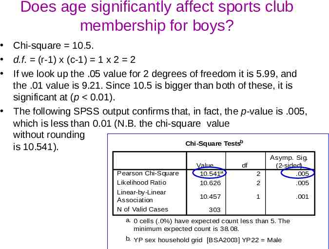
Does age significantly affect sports club membership for boys? Chi-square 10.5. d.f. (r-1) x (c-1) 1 x 2 2 If we look up the .05 value for 2 degrees of freedom it is 5.99, and the .01 value is 9.21. Since 10.5 is bigger than both of these, it is significant at (p 0.01). The following SPSS output confirms that, in fact, the p-value is .005, which is less than 0.01 (N.B. the chi-square value without rounding Chi-Square Testsb is 10.541). Pearson Chi-Square Likelihood Ratio Linear-by-Linear Association N of Valid Cases Value 10.541a 10.626 10.457 2 2 Asymp. Sig. (2-sided) .005 .005 1 .001 df 303 a. 0 cells (.0%) have expected count less than 5. The minimum expected count is 38.08. b. YP sex household grid [BSA2003] YP22 Male

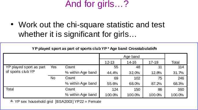
And for girls ? Work out the chi-square statistic and test whether it is significant for girls a YP played sport as part of sports club YP * Age band Crosstabulation YP played sport as part of sports club YP Yes No Total Count % within Age band Count % within Age band Count % within Age band a. YP sex household grid [BSA2003] YP22 Female 12-13 55 44.4% 69 55.6% 124 100.0% Age band 14-16 48 32.0% 102 68.0% 150 100.0% 17-19 11 12.8% 75 87.2% 86 100.0% Total 114 31.7% 246 68.3% 360 100.0%

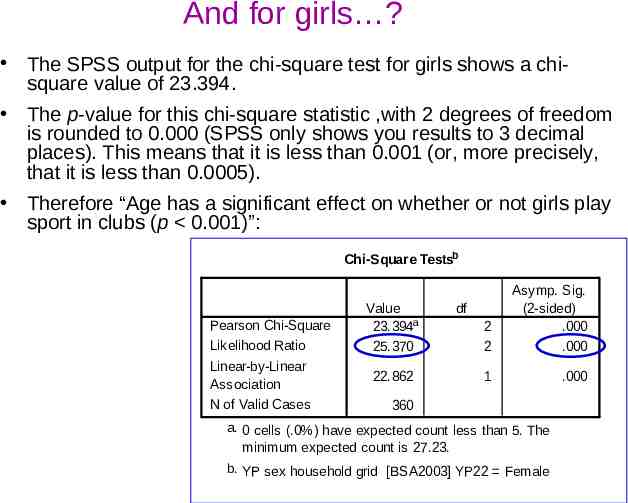
And for girls ? The SPSS output for the chi-square test for girls shows a chisquare value of 23.394. The p-value for this chi-square statistic ,with 2 degrees of freedom is rounded to 0.000 (SPSS only shows you results to 3 decimal places). This means that it is less than 0.001 (or, more precisely, that it is less than 0.0005). Therefore “Age has a significant effect on whether or not girls play sport in clubs (p 0.001)”: Chi-Square Testsb Pearson Chi-Square Likelihood Ratio Linear-by-Linear Association N of Valid Cases Value 23.394a 25.370 22.862 2 2 Asymp. Sig. (2-sided) .000 .000 1 .000 df 360 a. 0 cells (.0%) have expected count less than 5. The minimum expected count is 27.23. b. YP sex household grid [BSA2003] YP22 Female

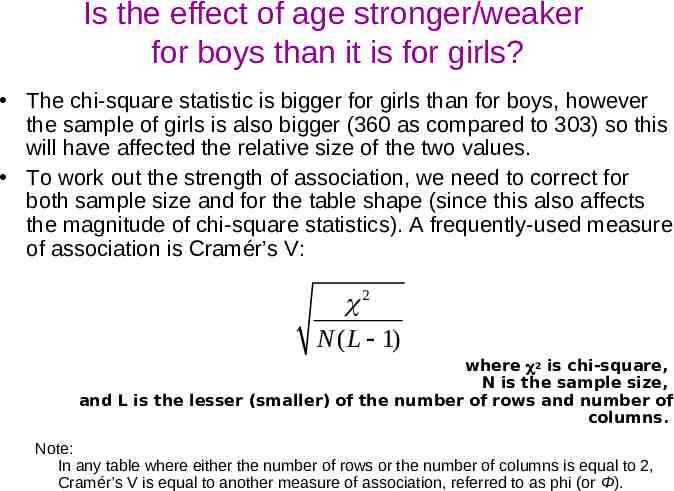
Is the effect of age stronger/weaker for boys than it is for girls? The chi-square statistic is bigger for girls than for boys, however the sample of girls is also bigger (360 as compared to 303) so this will have affected the relative size of the two values. To work out the strength of association, we need to correct for both sample size and for the table shape (since this also affects the magnitude of chi-square statistics). A frequently-used measure of association is Cramér’s V: 2 N ( L 1) where 2 is chi-square, N is the sample size, and L is the lesser (smaller) of the number of rows and number of columns. Note: In any table where either the number of rows or the number of columns is equal to 2, Cramér’s V is equal to another measure of association, referred to as phi (or Φ).

Comparing strength of association between age and involvement in sport for boys and for girls a YP played sport as part of sports club YP * Age band Crosstabulation Boys: YP played sport as part of sports club YP χ 10.541 Yes No 2 Total Count % within Age band Count % within Age band Count % within Age band 12-13 62 65.3% 33 34.7% 95 100.0% Age band 14-16 68 54.4% 57 45.6% 125 100.0% 17-19 34 41.0% 49 59.0% 83 100.0% Total 164 54.1% 139 45.9% 303 100.0% a. YP sex household grid [BSA2003] YP22 Male a YP played sport as part of sports club YP * Age band Crosstabulation Girls : YP played sport as part of sports club YP χ2 23.394 Yes No Total Count % within Age band Count % within Age band Count % within Age band 12-13 55 44.4% 69 55.6% 124 100.0% Age band 14-16 48 32.0% 102 68.0% 150 100.0% 17-19 11 12.8% 75 87.2% 86 100.0% Total 114 31.7% 246 68.3% 360 100.0% a. YP sex household grid [BSA2003] YP22 Female Cramér’s V values for the two tables are therefore: 2 N ( L 1) Boy s 10.5 0.186 303(2 1) Girls 23.9 0.258 360(2 1)

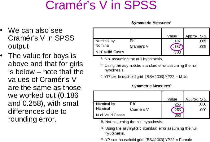
Cramér’s V in SPSS Symmetric Measuresc We can also see Cramér’s V in SPSS output The value for boys is above and that for girls is below – note that the values of Cramér’s V are the same as those we worked out (0.186 and 0.258), with small differences due to rounding error. Nominal by Nominal Phi Cramer's V N of Valid Cases Value .187 .187 303 Approx. Sig. .005 .005 a. Not assuming the null hypothesis. b. Using the asymptotic standard error assuming the null hypothesis. c. YP sex household grid [BSA2003] YP22 Male Symmetric Measuresc Nominal by Nominal Phi Cramer's V N of Valid Cases Value .255 .255 360 Approx. Sig. .000 .000 a. Not assuming the null hypothesis. b. Using the asymptotic standard error assuming the null hypothesis. c. YP sex household grid [BSA2003] YP22 Female

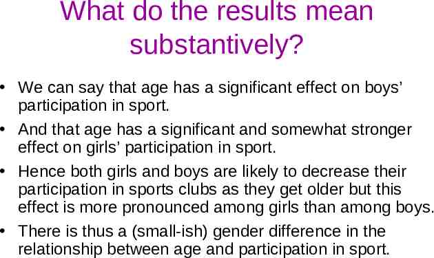
What do the results mean substantively? We can say that age has a significant effect on boys’ participation in sport. And that age has a significant and somewhat stronger effect on girls’ participation in sport. Hence both girls and boys are likely to decrease their participation in sports clubs as they get older but this effect is more pronounced among girls than among boys. There is thus a (small-ish) gender difference in the relationship between age and participation in sport.

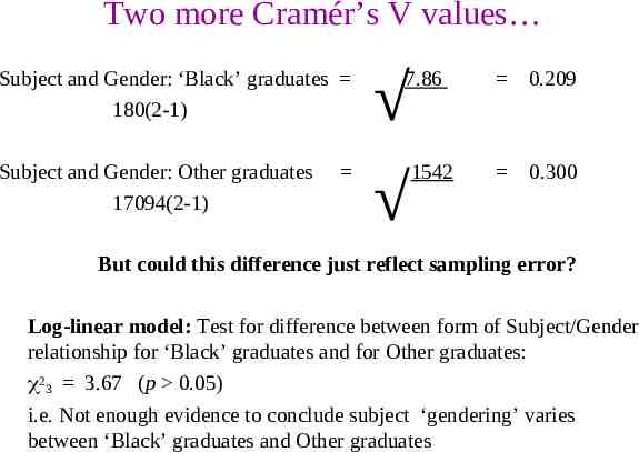
Two more Cramér’s V values Subject and Gender: ‘Black’ graduates 180(2-1) Subject and Gender: Other graduates 17094(2-1) 7.86 0.209 1542 0.300 But could this difference just reflect sampling error? Log-linear model: Test for difference between form of Subject/Gender relationship for ‘Black’ graduates and for Other graduates: 23 3.67 (p 0.05) i.e. Not enough evidence to conclude subject ‘gendering’ varies between ‘Black’ graduates and Other graduates