Descriptive Statistics The farthest most people ever get

Descriptive Statistics The farthest most people ever get

Descriptive Statistics Descriptive Statistics are Used by Researchers to Report on Populations and Samples In Sociology: Summary descriptions of measurements (variables) taken about a group of people By Summarizing Information, Descriptive Statistics Speed Up and Simplify Comprehension of a Group’s Characteristics

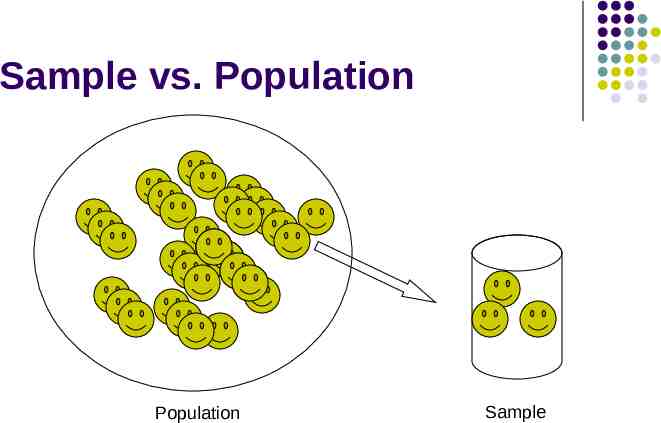
Sample vs. Population Population Sample

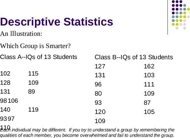
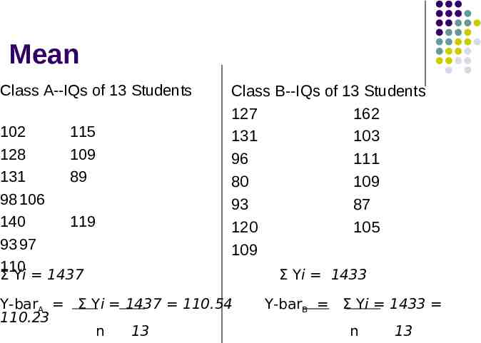
Descriptive Statistics An Illustration: Which Group is Smarter? Class A--IQs of 13 Students 102 115 128 109 131 89 98 106 140 119 93 97 110 Each individual may be different. Class B--IQs of 13 Students 127 162 131 103 96 111 80 109 93 87 120 105 109 If you try to understand a group by remembering the qualities of each member, you become overwhelmed and fail to understand the group.

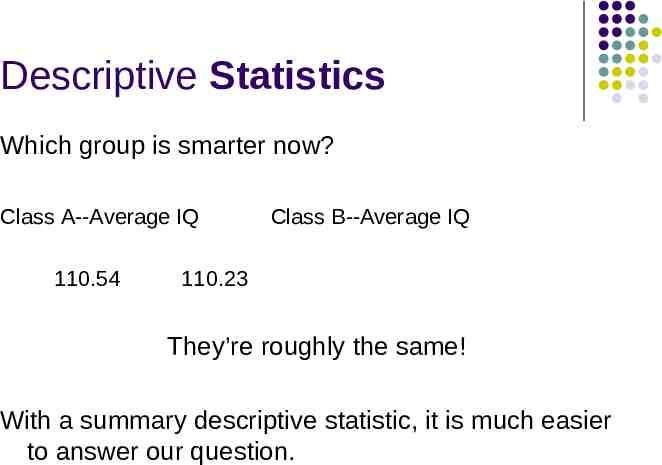
Descriptive Statistics Which group is smarter now? Class A--Average IQ 110.54 Class B--Average IQ 110.23 They’re roughly the same! With a summary descriptive statistic, it is much easier to answer our question.

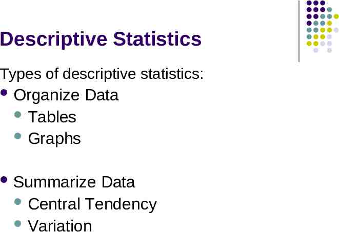
Descriptive Statistics Types of descriptive statistics: Organize Data Tables Graphs Summarize Data Central Tendency Variation

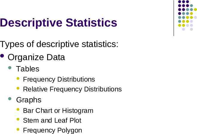
Descriptive Statistics Types of descriptive statistics: Organize Data Tables Frequency Distributions Relative Frequency Distributions Graphs Bar Chart or Histogram Stem and Leaf Plot Frequency Polygon

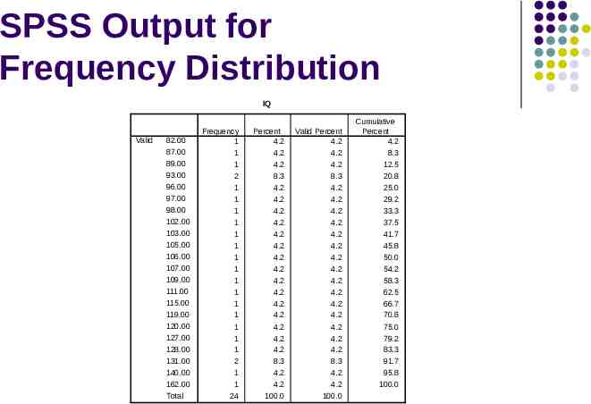
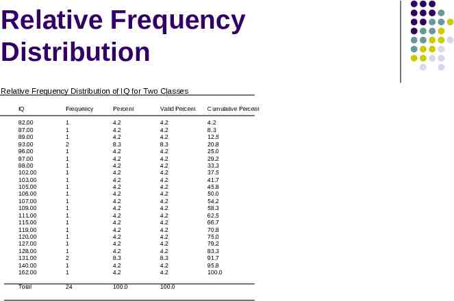
SPSS Output for Frequency Distribution IQ Valid 82.00 87.00 89.00 93.00 96.00 97.00 98.00 102.00 103.00 105.00 106.00 107.00 109.00 111.00 115.00 119.00 120.00 127.00 128.00 131.00 140.00 162.00 Total Frequency 1 1 1 2 1 1 1 1 1 1 1 1 1 1 1 1 1 1 1 2 1 1 24 Percent 4.2 4.2 4.2 8.3 4.2 4.2 4.2 4.2 4.2 4.2 4.2 4.2 4.2 4.2 4.2 4.2 4.2 4.2 4.2 8.3 4.2 4.2 100.0 Valid Percent 4.2 4.2 4.2 8.3 4.2 4.2 4.2 4.2 4.2 4.2 4.2 4.2 4.2 4.2 4.2 4.2 4.2 4.2 4.2 8.3 4.2 4.2 100.0 Cumulative Percent 4.2 8.3 12.5 20.8 25.0 29.2 33.3 37.5 41.7 45.8 50.0 54.2 58.3 62.5 66.7 70.8 75.0 79.2 83.3 91.7 95.8 100.0

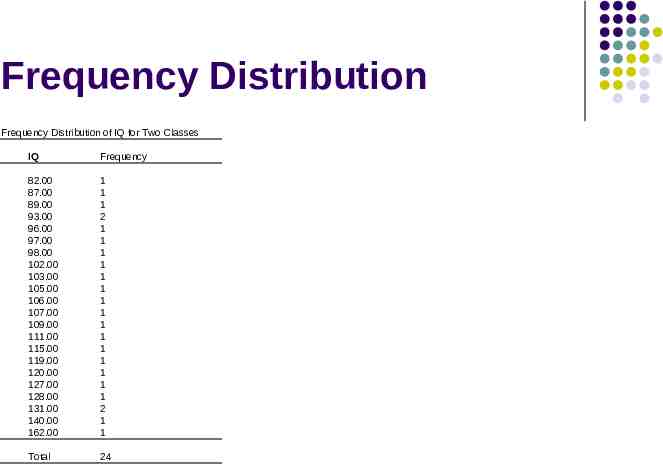
Frequency Distribution Frequency Distribution of IQ for Two Classes IQ Frequency 82.00 87.00 89.00 93.00 96.00 97.00 98.00 102.00 103.00 105.00 106.00 107.00 109.00 111.00 115.00 119.00 120.00 127.00 128.00 131.00 140.00 162.00 1 1 1 2 1 1 1 1 1 1 1 1 1 1 1 1 1 1 1 2 1 1 Total 24

Relative Frequency Distribution Relative Frequency Distribution of IQ for Two Classes IQ Frequency Percent Valid Percent Cumulative Percent 82.00 87.00 89.00 93.00 96.00 97.00 98.00 102.00 103.00 105.00 106.00 107.00 109.00 111.00 115.00 119.00 120.00 127.00 128.00 131.00 140.00 162.00 1 1 1 2 1 1 1 1 1 1 1 1 1 1 1 1 1 1 1 2 1 1 4.2 4.2 4.2 8.3 4.2 4.2 4.2 4.2 4.2 4.2 4.2 4.2 4.2 4.2 4.2 4.2 4.2 4.2 4.2 8.3 4.2 4.2 4.2 4.2 4.2 8.3 4.2 4.2 4.2 4.2 4.2 4.2 4.2 4.2 4.2 4.2 4.2 4.2 4.2 4.2 4.2 8.3 4.2 4.2 4.2 8.3 12.5 20.8 25.0 29.2 33.3 37.5 41.7 45.8 50.0 54.2 58.3 62.5 66.7 70.8 75.0 79.2 83.3 91.7 95.8 100.0 Total 24 100.0 100.0

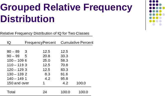
Grouped Relative Frequency Distribution Relative Frequency Distribution of IQ for Two Classes IQ FrequencyPercent Cumulative Percent 80 – 89 3 90 – 99 5 100 – 109 6 110 – 119 3 120 – 129 3 130 – 139 2 140 – 149 1 150 and over 12.5 20.8 25.0 12.5 12.5 8.3 4.2 1 12.5 33.3 58.3 70.8 83.3 91.6 95.8 4.2 Total 24 100.0 100.0 100.0

SPSS Output for Histogram

Histogram

Bar Graph

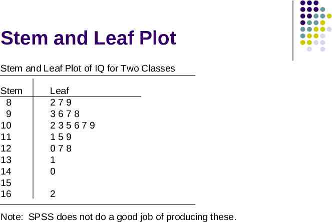
Stem and Leaf Plot Stem and Leaf Plot of IQ for Two Classes Stem 8 9 10 11 12 13 14 15 16 Leaf 279 3678 235679 159 078 1 0 2 Note: SPSS does not do a good job of producing these.

SPSS Output of a Frequency Polygon

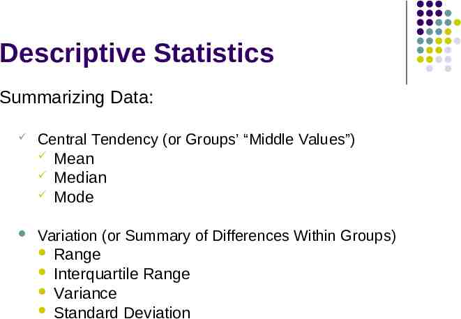
Descriptive Statistics Summarizing Data: Central Tendency (or Groups’ “Middle Values”) Mean Median Mode Variation (or Summary of Differences Within Groups) Range Interquartile Range Variance Standard Deviation

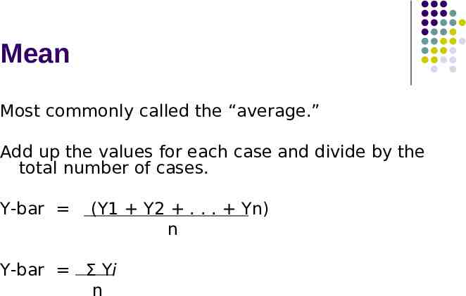
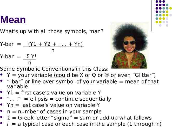
Mean Most commonly called the “average.” Add up the values for each case and divide by the total number of cases. Y-bar (Y1 Y2 . . . Yn) n Y-bar Σ Yi n

Mean What’s up with all those symbols, man? Y-bar (Y1 Y2 . . . Yn) n Y-bar Σ Yi n Some Symbolic Conventions in this Class: Y your variable (could be X or Q or or even “Glitter”) “-bar” or line over symbol of your variable mean of that variable Y1 first case’s value on variable Y “. . .” ellipsis continue sequentially Yn last case’s value on variable Y n number of cases in your sample Σ Greek letter “sigma” sum or add up what follows i a typical case or each case in the sample (1 through n)

Mean Class A--IQs of 13 Students 102 128 131 98 106 140 93 97 110 115 109 89 119 Class B--IQs of 13 Students 127 162 131 103 96 111 80 109 93 87 120 105 109 Σ Yi 1437 Y-barA Σ Yi 1437 110.54 110.23 n 13 Σ Yi 1433 Y-barB Σ Yi 1433 n 13

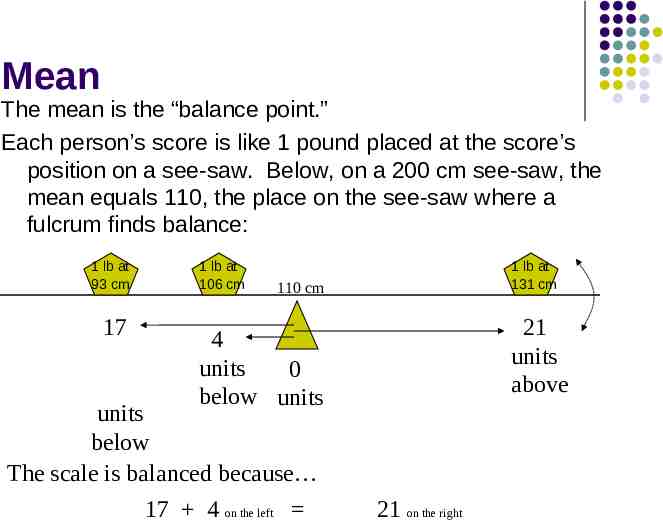
Mean The mean is the “balance point.” Each person’s score is like 1 pound placed at the score’s position on a see-saw. Below, on a 200 cm see-saw, the mean equals 110, the place on the see-saw where a fulcrum finds balance: 1 lb at 93 cm 17 1 lb at 106 cm 1 lb at 131 cm 110 cm 21 units above 4 units 0 below units units below The scale is balanced because 17 4 on the left 21 on the right

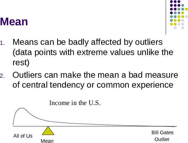
Mean 1. 2. Means can be badly affected by outliers (data points with extreme values unlike the rest) Outliers can make the mean a bad measure of central tendency or common experience Income in the U.S. All of Us Mean Bill Gates Outlier

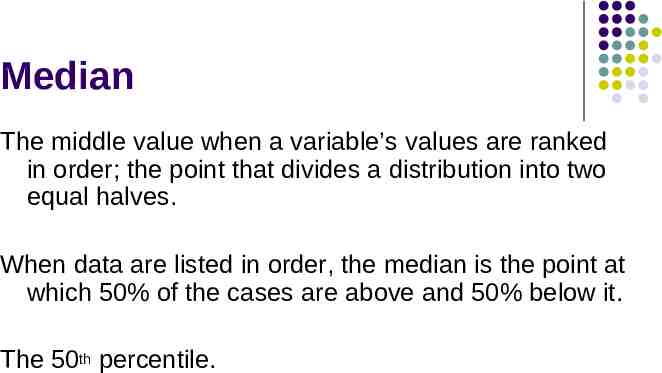
Median The middle value when a variable’s values are ranked in order; the point that divides a distribution into two equal halves. When data are listed in order, the median is the point at which 50% of the cases are above and 50% below it. The 50th percentile.

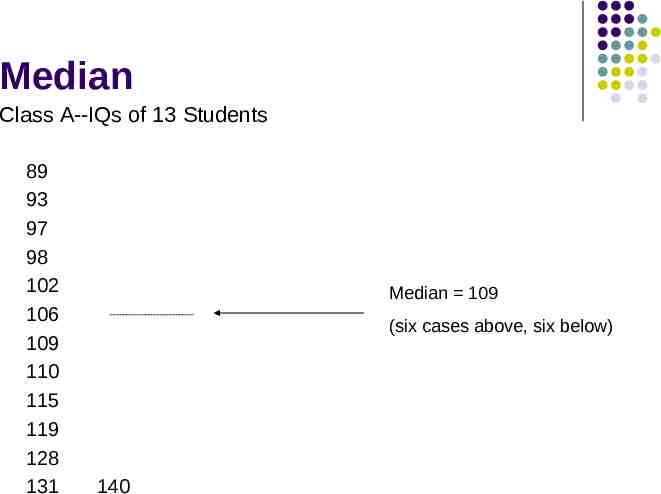
Median Class A--IQs of 13 Students 89 93 97 98 102 106 109 110 115 119 128 131 Median 109 (six cases above, six below) 140

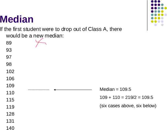
Median If the first student were to drop out of Class A, there would be a new median: 89 93 97 98 102 106 109 110 115 119 128 131 140 Median 109.5 109 110 219/2 109.5 (six cases above, six below)

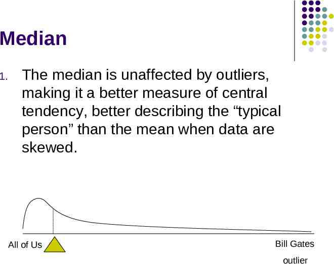
Median 1. The median is unaffected by outliers, making it a better measure of central tendency, better describing the “typical person” than the mean when data are skewed. All of Us Bill Gates outlier

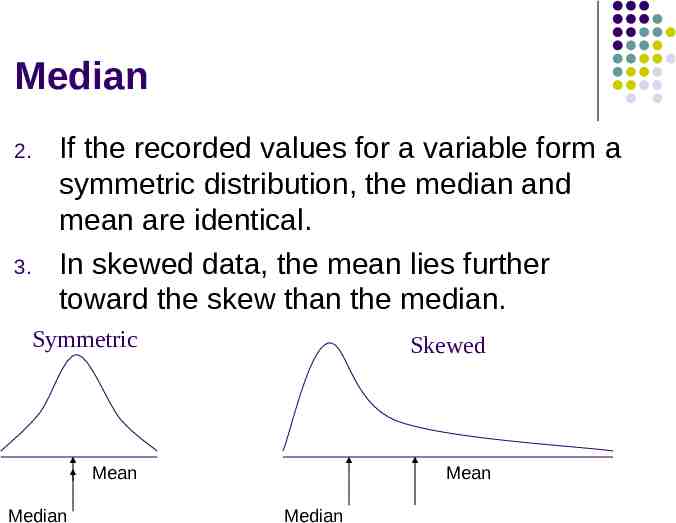
Median 2. 3. If the recorded values for a variable form a symmetric distribution, the median and mean are identical. In skewed data, the mean lies further toward the skew than the median. Symmetric Skewed Mean Mean Median Median

Median The middle score or measurement in a set of ranked scores or measurements; the point that divides a distribution into two equal halves. Data are listed in order—the median is the point at which 50% of the cases are above and 50% below. The 50th percentile.

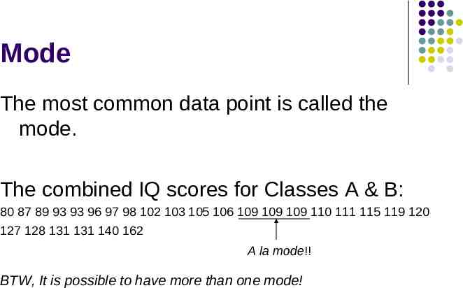
Mode The most common data point is called the mode. The combined IQ scores for Classes A & B: 80 87 89 93 93 96 97 98 102 103 105 106 109 109 109 110 111 115 119 120 127 128 131 131 140 162 A la mode!! BTW, It is possible to have more than one mode!

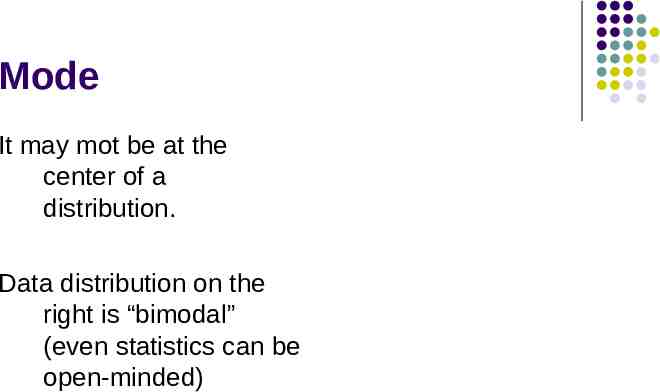
Mode It may mot be at the center of a distribution. Data distribution on the right is “bimodal” (even statistics can be open-minded)

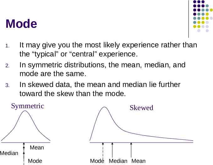
Mode It may give you the most likely experience rather than the “typical” or “central” experience. In symmetric distributions, the mean, median, and mode are the same. In skewed data, the mean and median lie further toward the skew than the mode. 1. 2. 3. Symmetric Median Skewed Mean Mode Mode Median Mean

Descriptive Statistics Summarizing Data: Central Tendency (or Groups’ “Middle Values”) Mean Median Mode Variation (or Summary of Differences Within Groups) Range Interquartile Range Variance Standard Deviation

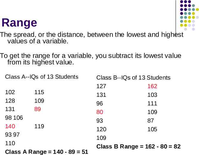
Range The spread, or the distance, between the lowest and highest values of a variable. To get the range for a variable, you subtract its lowest value from its highest value. Class A--IQs of 13 Students 102 115 128 109 131 89 98 106 140 119 93 97 110 Class A Range 140 - 89 51 Class B--IQs of 13 Students 127 162 131 103 96 111 80 109 93 87 120 105 109 Class B Range 162 - 80 82

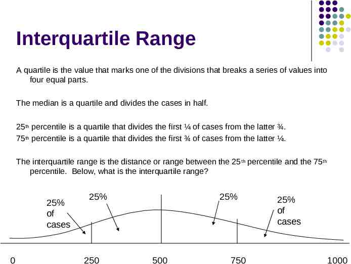
Interquartile Range A quartile is the value that marks one of the divisions that breaks a series of values into four equal parts. The median is a quartile and divides the cases in half. 25th percentile is a quartile that divides the first ¼ of cases from the latter ¾. 75th percentile is a quartile that divides the first ¾ of cases from the latter ¼. The interquartile range is the distance or range between the 25 th percentile and the 75th percentile. Below, what is the interquartile range? 25% of cases 0 25% 250 25% 500 750 25% of cases 1000

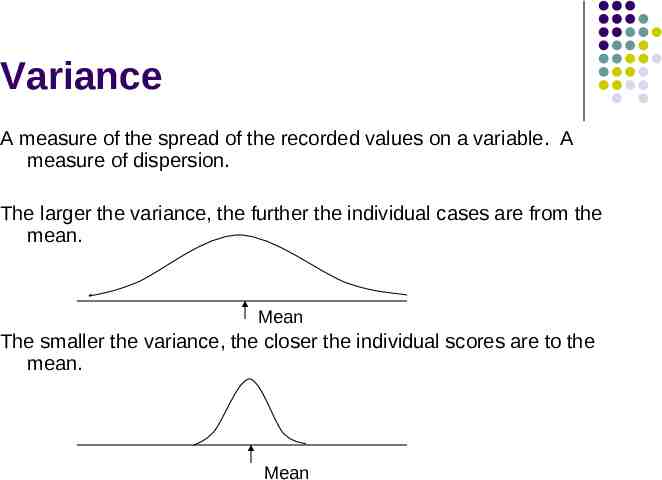
Variance A measure of the spread of the recorded values on a variable. A measure of dispersion. The larger the variance, the further the individual cases are from the mean. Mean The smaller the variance, the closer the individual scores are to the mean. Mean

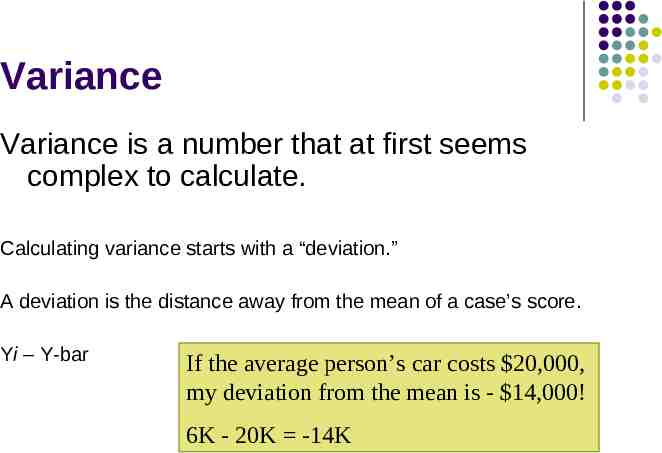
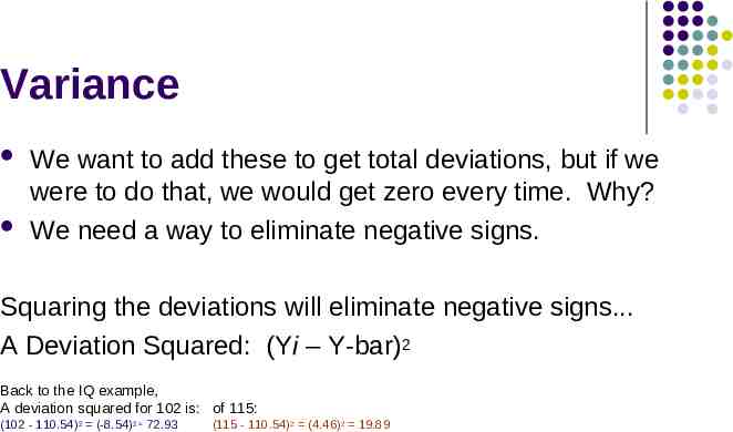
Variance Variance is a number that at first seems complex to calculate. Calculating variance starts with a “deviation.” A deviation is the distance away from the mean of a case’s score. Yi – Y-bar If the average person’s car costs 20,000, my deviation from the mean is - 14,000! 6K - 20K -14K

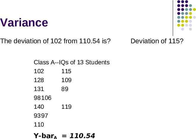
Variance The deviation of 102 from 110.54 is? Class A--IQs of 13 Students 102 115 128 109 131 89 98 106 140 119 93 97 110 Y-barA 110.54 Deviation of 115?

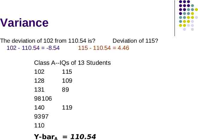
Variance The deviation of 102 from 110.54 is? Deviation of 115? 102 - 110.54 -8.54 115 - 110.54 4.46 Class A--IQs of 13 Students 102 115 128 109 131 89 98 106 140 119 93 97 110 Y-barA 110.54

Variance We want to add these to get total deviations, but if we were to do that, we would get zero every time. Why? We need a way to eliminate negative signs. Squaring the deviations will eliminate negative signs. A Deviation Squared: (Yi – Y-bar)2 Back to the IQ example, A deviation squared for 102 is: of 115: (102 - 110.54)2 (-8.54)2 72.93 (115 - 110.54)2 (4.46)2 19.89

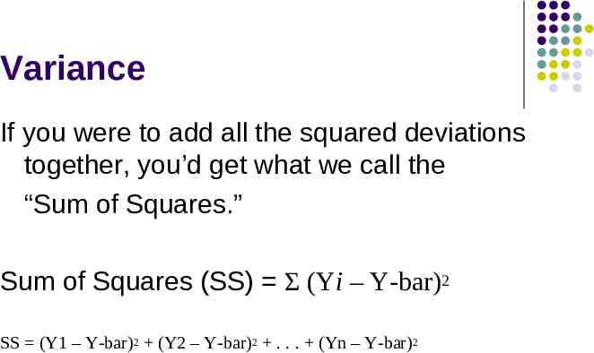
Variance If you were to add all the squared deviations together, you’d get what we call the “Sum of Squares.” Sum of Squares (SS) Σ (Yi – Y-bar)2 SS (Y1 – Y-bar)2 (Y2 – Y-bar)2 . . . (Yn – Y-bar)2

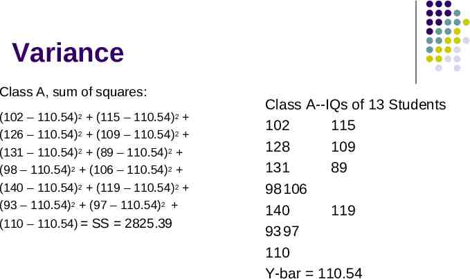
Variance Class A, sum of squares: (102 – 110.54) (115 – 110.54) (126 – 110.54)2 (109 – 110.54)2 (131 – 110.54)2 (89 – 110.54)2 (98 – 110.54)2 (106 – 110.54)2 (140 – 110.54)2 (119 – 110.54)2 (93 – 110.54)2 (97 – 110.54)2 2 (110 – 110.54) SS 2825.39 2 Class A--IQs of 13 Students 102 115 128 109 131 89 98 106 140 119 93 97 110 Y-bar 110.54

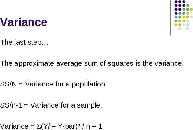
Variance The last step The approximate average sum of squares is the variance. SS/N Variance for a population. SS/n-1 Variance for a sample. Variance Σ(Yi – Y-bar)2 / n – 1

Variance For Class A, Variance 2825.39 / n - 1 2825.39 / 12 235.45 How helpful is that?

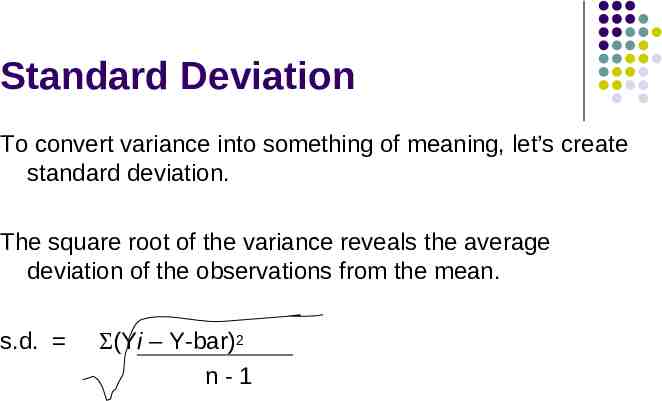
Standard Deviation To convert variance into something of meaning, let’s create standard deviation. The square root of the variance reveals the average deviation of the observations from the mean. s.d. Σ(Yi – Y-bar)2 n-1

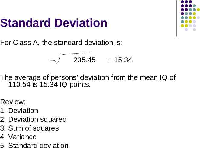
Standard Deviation For Class A, the standard deviation is: 235.45 15.34 The average of persons’ deviation from the mean IQ of 110.54 is 15.34 IQ points. Review: 1. Deviation 2. Deviation squared 3. Sum of squares 4. Variance 5. Standard deviation

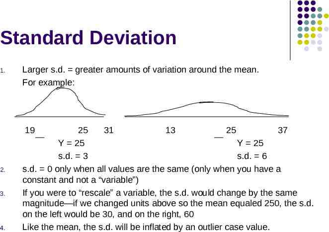
Standard Deviation 1. Larger s.d. greater amounts of variation around the mean. For example: 19 2. 3. 4. 25 31 13 25 37 Y 25 Y 25 s.d. 3 s.d. 6 s.d. 0 only when all values are the same (only when you have a constant and not a “variable”) If you were to “rescale” a variable, the s.d. would change by the same magnitude—if we changed units above so the mean equaled 250, the s.d. on the left would be 30, and on the right, 60 Like the mean, the s.d. will be inflated by an outlier case value.

Standard Deviation Note about computational formulas: Your book provides a useful short-cut formula for computing the variance and standard deviation. This is intended to make hand calculations as quick as possible. They obscure the conceptual understanding of our statistics. SPSS and the computer are “computational formulas” now.

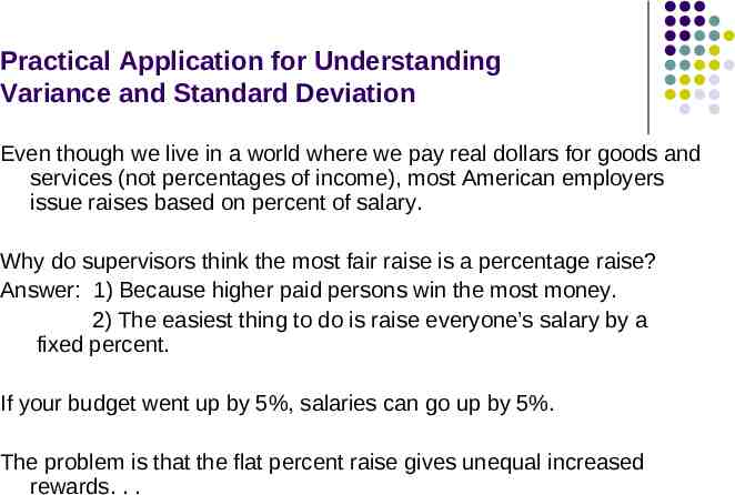
Practical Application for Understanding Variance and Standard Deviation Even though we live in a world where we pay real dollars for goods and services (not percentages of income), most American employers issue raises based on percent of salary. Why do supervisors think the most fair raise is a percentage raise? Answer: 1) Because higher paid persons win the most money. 2) The easiest thing to do is raise everyone’s salary by a fixed percent. If your budget went up by 5%, salaries can go up by 5%. The problem is that the flat percent raise gives unequal increased rewards. . .

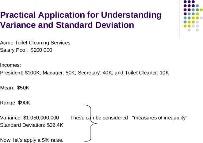
Practical Application for Understanding Variance and Standard Deviation Acme Toilet Cleaning Services Salary Pool: 200,000 Incomes: President: 100K; Manager: 50K; Secretary: 40K; and Toilet Cleaner: 10K Mean: 50K Range: 90K Variance: 1,050,000,000 Standard Deviation: 32.4K Now, let’s apply a 5% raise. These can be considered “measures of inequality”

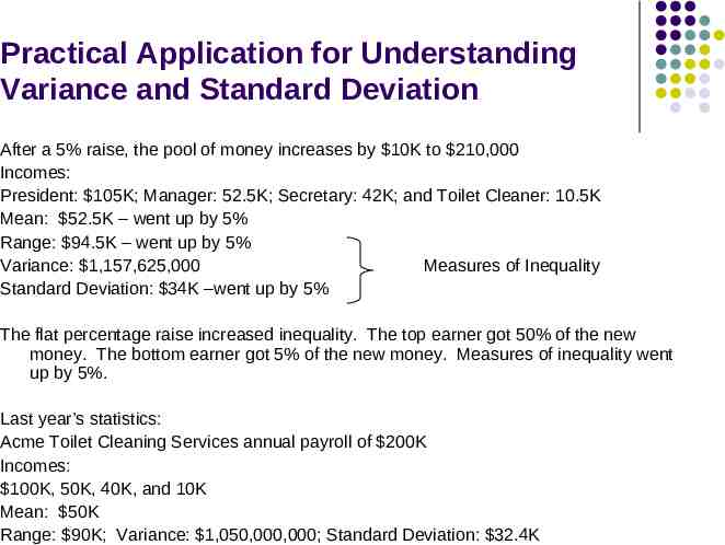
Practical Application for Understanding Variance and Standard Deviation After a 5% raise, the pool of money increases by 10K to 210,000 Incomes: President: 105K; Manager: 52.5K; Secretary: 42K; and Toilet Cleaner: 10.5K Mean: 52.5K – went up by 5% Range: 94.5K – went up by 5% Variance: 1,157,625,000 Measures of Inequality Standard Deviation: 34K –went up by 5% The flat percentage raise increased inequality. The top earner got 50% of the new money. The bottom earner got 5% of the new money. Measures of inequality went up by 5%. Last year’s statistics: Acme Toilet Cleaning Services annual payroll of 200K Incomes: 100K, 50K, 40K, and 10K Mean: 50K Range: 90K; Variance: 1,050,000,000; Standard Deviation: 32.4K

Practical Application for Understanding Variance and Standard Deviation The flat percentage raise increased inequality. The top earner got 50% of the new money. The bottom earner got 5% of the new money. Inequality increased by 5%. Since we pay for goods and services in real dollars, not in percentages, there are substantially more new things the top earners can purchase compared with the bottom earner for the rest of their employment years. Acme Toilet Cleaning Services is giving the earners 5,000, 2,500, 2,000, and 500 more respectively each and every year forever. What does this mean in terms of compounding raises? Acme is essentially saying: “Each year we’ll buy you a new TV, in addition to everything else you buy, here’s what you’ll get:”

Practical Application for Understanding Variance and Standard Deviation Toilet Cleaner Secretary Manager President The gap between the rich and poor expands. This is why some progressive organizations give a percentage raise with a flat increase for lowest wage earners. For example, 5% or 1,000, whichever is greater.

Descriptive Statistics Summarizing Data: Central Tendency (or Groups’ “Middle Values”) Mean Median Mode Variation (or Summary of Differences Within Groups) Range Interquartile Range Variance Standard Deviation Wait! There’s more

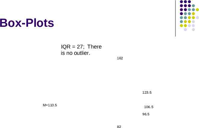
Box-Plots A way to graphically portray almost all the descriptive statistics at once is the box-plot. A box-plot shows: Upper and lower quartiles Mean Median Range Outliers (1.5 IQR)

Box-Plots IQR 27; There is no outlier. 162 123.5 M 110.5 106.5 96.5 82

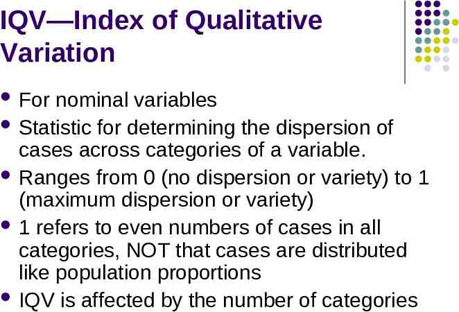
IQV—Index of Qualitative Variation For nominal variables Statistic for determining the dispersion of cases across categories of a variable. Ranges from 0 (no dispersion or variety) to 1 (maximum dispersion or variety) 1 refers to even numbers of cases in all categories, NOT that cases are distributed like population proportions IQV is affected by the number of categories

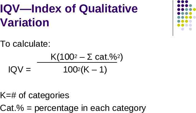
IQV—Index of Qualitative Variation To calculate: IQV K(1002 – Σ cat.%2) 1002(K – 1) K # of categories Cat.% percentage in each category

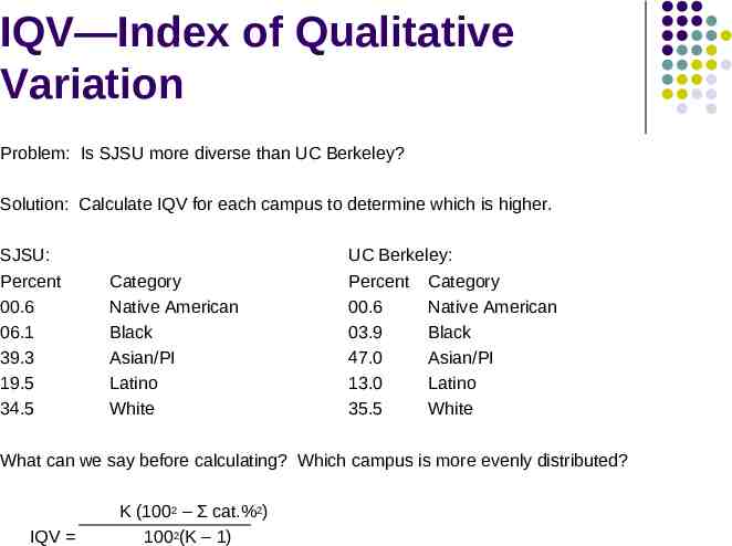
IQV—Index of Qualitative Variation Problem: Is SJSU more diverse than UC Berkeley? Solution: Calculate IQV for each campus to determine which is higher. SJSU: Percent 00.6 06.1 39.3 19.5 34.5 Category Native American Black Asian/PI Latino White UC Berkeley: Percent Category 00.6 Native American 03.9 Black 47.0 Asian/PI 13.0 Latino 35.5 White What can we say before calculating? Which campus is more evenly distributed? IQV K (1002 – Σ cat.%2) 1002(K – 1)

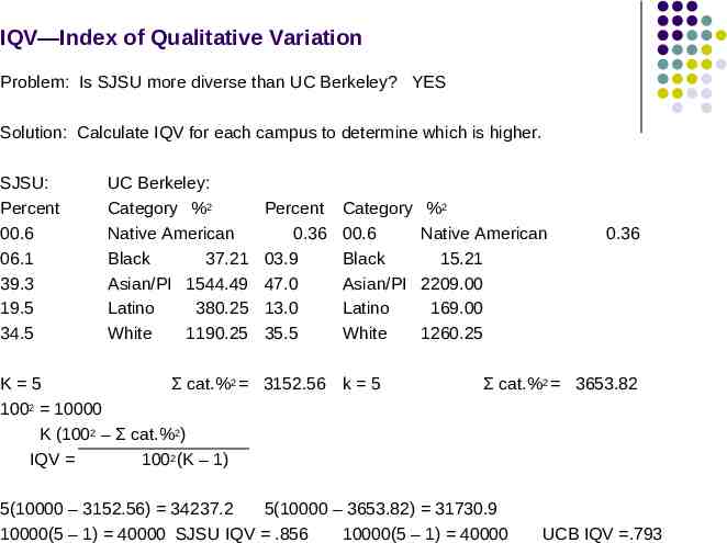
IQV—Index of Qualitative Variation Problem: Is SJSU more diverse than UC Berkeley? YES Solution: Calculate IQV for each campus to determine which is higher. SJSU: Percent 00.6 06.1 39.3 19.5 34.5 UC Berkeley: Category %2 Native American Black 37.21 Asian/PI 1544.49 Latino 380.25 White 1190.25 Percent 0.36 03.9 47.0 13.0 35.5 Category 00.6 Black Asian/PI Latino White K 5 Σ cat.%2 3152.56 k 5 1002 10000 K (1002 – Σ cat.%2) IQV 1002(K – 1) %2 Native American 15.21 2209.00 169.00 1260.25 0.36 Σ cat.%2 3653.82 5(10000 – 3152.56) 34237.2 5(10000 – 3653.82) 31730.9 10000(5 – 1) 40000 SJSU IQV .856 10000(5 – 1) 40000 UCB IQV .793

Descriptive Statistics Now you are qualified use descriptive statistics! Questions?