Consumer Theory Dr. Jennifer P. Wissink 2011 John M. Abowd and

Consumer Theory Dr. Jennifer P. Wissink 2011 John M. Abowd and Jennifer P. Wissink, all rights reserved.

Consumer Theory Study of how people use their limited means to make purposeful choices. Assumes that consumers understand what they like/dislike as their objective (preferences) and the prices (opportunity costs) associated with choices they can make. Assumes that consumers consider the alternatives and choose to maximize their objective subject to their constraints.

Why Don’t We Just Use The Demand Curve? Recall: The “Market Demand Function & Curve” for a single good aggregates and summarizes all market consumers’ intended purchases. “Consumer Theory” allows us to: – Build the market demand function & curve from scratch, that is, from its core “ingredients.” – Use the consumer theory model to address issues not adequately explained via reference to the summarized and aggregated model.

Two Components Of Consumer Demand Opportunities: – What can the consumer afford? – What are the consumption possibilities? – Summarized by the budget constraint Preferences: – What does the consumer like? – How much does a consumer like a good? – How would a consumer willingly trade off one good for another? – Summarized by indifference curve maps and the utility function

Ultimate Goal We are going to carefully study the demand system for two consumers (Maryclaire and Katie) who consume only two goods (beans and carrots). For each good and each consumer, the theory produces a demand function: – Demand function for beans: Bi fB(PB, PC, I) i Maryclaire, Katie – Demand function for carrots: Ci fC(PB, PC, I) i Maryclaire, Katie – where PB is the price of beans, PC is the price of carrots, and I is the consumer i’s income. When we properly aggregate the two consumers’ demand equations we get the market demand equations, one for beans and one for carrots.

What Is A Budget Constraint? A budget constraint shows the consumer’s purchase opportunities as every combination of two goods that can be bought at given prices totally using up a given amount of income. The mathematical expression for the budget constraint is: – Income Price Beans x Beans Price Carrots x Carrots – In symbols » I PBB PCC where I is the consumer’s income. PB is the price of beans, B is pounds of beans, PC is the price of carrots, and C is pounds of carrots.

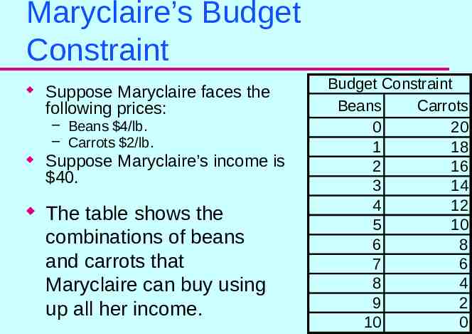
Maryclaire’s Budget Constraint Suppose Maryclaire faces the following prices: – Beans 4/lb. – Carrots 2/lb. Suppose Maryclaire’s income is 40. The table shows the combinations of beans and carrots that Maryclaire can buy using up all her income. Budget Constraint Beans Carrots 0 20 1 18 2 16 3 14 4 12 5 10 6 8 7 6 8 4 9 2 10 0

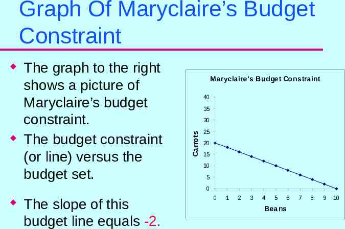
Graph Of Maryclaire’s Budget Constraint The graph to the right shows a picture of Maryclaire’s budget constraint. The budget constraint (or line) versus the budget set. M aryclaire's Budget Constraint 40 35 30 Carrots 25 20 15 10 5 0 The slope of this budget line equals -2. 0 1 2 3 4 5 6 Beans 7 8 9 10

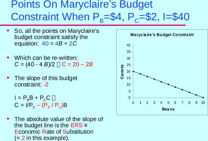
Points On Maryclaire’s Budget Constraint When PB 4, PC 2, I 40 So, all the points on Maryclaire’s budget constraint satisfy the equation: 40 4B 2C M aryclaire's Budget Constraint 40 35 Which can be re-written: C (40 - 4 B)/2 C 20 – 2B The slope of this budget constraint: -2 30 Carrots 25 20 15 10 5 I PBB PCC C I/PC – (PB / PC)B The absolute value of the slope of the budget line is the ERS Economic Rate of Substitution ( 2 in this example). 0 0 1 2 3 4 5 6 Beans 7 8 9 10

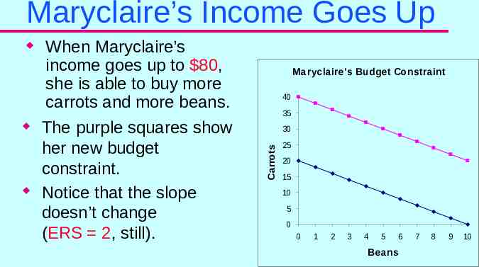
Maryclaire’s Income Goes Up When Maryclaire’s income goes up to 80, she is able to buy more carrots and more beans. The purple squares show her new budget constraint. Notice that the slope doesn’t change (ERS 2, still). M aryclaire's Budget Constraint 40 35 30 Carrots 25 20 15 10 5 0 0 1 2 3 4 5 6 Beans 7 8 9 10

Maryclaire Faces New Prices Now, suppose that the price of beans falls to 2/lb. and the price of carrots remains 2/lb. and I 40. The purple squares show the new budget constraint. Notice that the slope is now -2/2 -1 (ERS 1). M aryclaire's Budget Constraint 40 35 30 Carrots 25 20 15 10 5 0 0 1 2 3 4 5 6 Beans 7 8 9 10

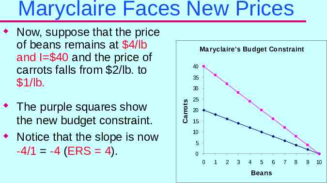
Maryclaire Faces New Prices Now, suppose that the price of beans remains at 4/lb and I 40 and the price of carrots falls from 2/lb. to 1/lb. The purple squares show the new budget constraint. Notice that the slope is now -4/1 -4 (ERS 4). M aryclaire's Budget Constraint 40 35 30 Carrots 25 20 15 10 5 0 0 1 2 3 4 5 6 Beans 7 8 9 10

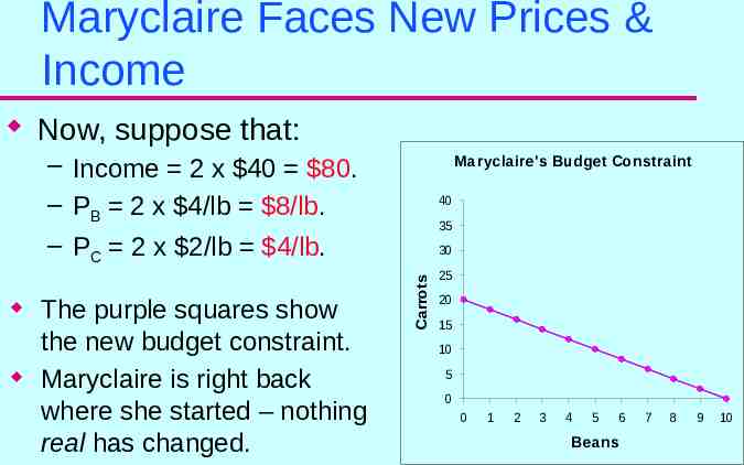
Maryclaire Faces New Prices & Income Now, suppose that: M aryclaire's Budget Constraint – Income 2 x 40 80. – PB 2 x 4/lb 8/lb. – PC 2 x 2/lb 4/lb. The purple squares show the new budget constraint. Maryclaire is right back where she started – nothing real has changed. 35 30 Carrots 40 25 20 15 10 5 0 0 1 2 3 4 5 6 Beans 7 8 9 10

Budget Line Gymnastics What have we done with the budget constraint: – An increase in income only. – A decrease in the price of beans only. – A decrease in the price of carrots only. Income doubles as do the prices of beans and carrots. – Maryclaire’s “real income” has not changed. – Real income increases when the budget line moves right (out). – Real income decreases when the budget line moves left (in). Changes in the price of beans relative to the price of carrots change the ERS, the slope of the budget line.

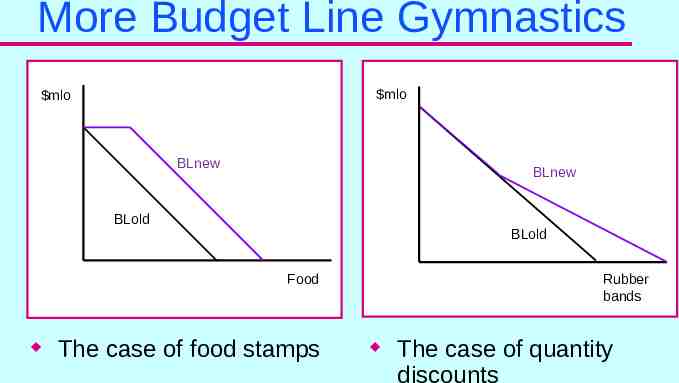
More Budget Line Gymnastics mlo mlo BLnew BLnew BLold BLold Food The case of food stamps Rubber bands The case of quantity discounts

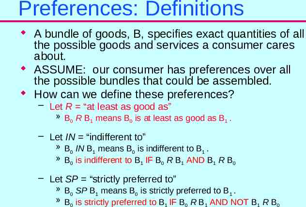
Preferences: Definitions A bundle of goods, B, specifies exact quantities of all the possible goods and services a consumer cares about. ASSUME: our consumer has preferences over all the possible bundles that could be assembled. How can we define these preferences? – Let R “at least as good as” » B0 R B1 means B0 is at least as good as B1 . – Let IN “indifferent to” » B0 IN B1 means B0 is indifferent to B1 . » B0 is indifferent to B1 IF B0 R B1 AND B1 R B0 – Let SP “strictly preferred to” » B0 SP B1 means B0 is strictly preferred to B1 . » B0 is strictly preferred to B1 IF B0 R B1 AND NOT B1 R B0

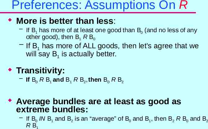
Preferences: Assumptions On R More is better than less: – If B1 has more of at least one good than B0 (and no less of any other good), then B1 R B0 – If B1 has more of ALL goods, then let’s agree that we will say B1 is actually better. Transitivity: – If B0 R B1 and B1 R B2, then B0 R B2 Average bundles are at least as good as extreme bundles: – If B0 IN B1 and B2 is an “average” of B0 and B1, then B2 R B0 and B2 R B1

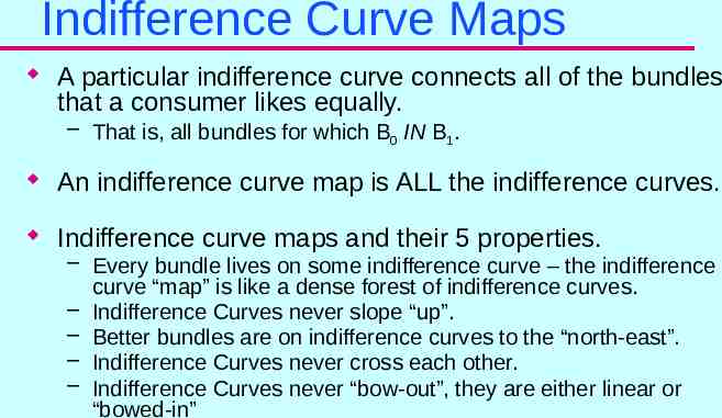
Indifference Curve Maps A particular indifference curve connects all of the bundles that a consumer likes equally. – That is, all bundles for which B0 IN B1. An indifference curve map is ALL the indifference curves. Indifference curve maps and their 5 properties. – Every bundle lives on some indifference curve – the indifference curve “map” is like a dense forest of indifference curves. – Indifference Curves never slope “up”. – Better bundles are on indifference curves to the “north-east”. – Indifference Curves never cross each other. – Indifference Curves never “bow-out”, they are either linear or “bowed-in”

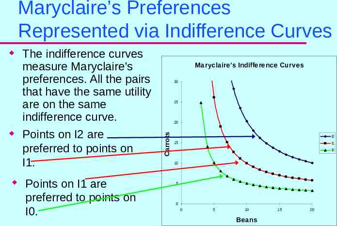
Maryclaire’s Preferences Represented via Indifference Curves The indifference curves measure Maryclaire’s preferences. All the pairs that have the same utility are on the same indifference curve. Points on I2 are preferred to points on I1. Points on I1 are preferred to points on I0. M aryclaire's Indifference Curves 30 25 20 Carrots I2 15 I1 I0 10 5 0 0 5 10 Beans 15 20

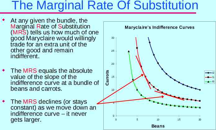
The Marginal Rate Of Substitution At any given the bundle, the Marginal Rate of Substitution (MRS) tells us how much of one good Maryclaire would willingly trade for an extra unit of the other good and remain indifferent. M aryclaire's Indifference Curves 30 25 The MRS equals the absolute value of the slope of the indifference curve at a bundle of beans and carrots. The MRS declines (or stays constant) as we move down an indifference curve – it never gets larger. Carrots 20 I2 15 I1 I0 10 5 0 0 5 10 Beans 15 20

From Preferences To Utility Utility is the way economists describe and sometimes measure preferences. Among two bundles, the one with the higher utility is the preferred bundle. If two bundles generate the same satisfaction then they have the same utility and we say that the consumer is indifferent between the two bundles.

Historical Note: What’s A Util? 19th Century Cardinalists – William Stanley Jevons 20th Century Ordinalists – Sir John Hicks

The Consumer Theory Problem: What Bundle Of Beans & Carrots? The optimal amount of beans and carrots to consume is the amount that maximizes utility subject to the budget constraint. The formal problem: Choose a bundle of (Beans, Carrots) to maximize u u(Beans, Carrots) subject to PBB PCC I

How To Find The Best Bundle Utility is at a maximum when: – all income is allocated to the goods you derive utility from AND – there is no way to transfer income from one good to another and make yourself any better off. » you are on the highest indifference curve you can possibly be on, and still on the budget line. » the slope of the indifference curve is equal to the slope of the budget constraint MRS ERS

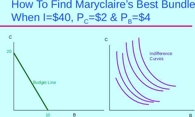
How To Find Maryclaire’s Best Bundle When I 40, PC 2 & PB 4 C C 20 Indifference Curves Budget Line 10 B B

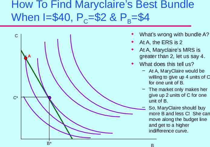
How To Find Maryclaire’s Best Bundle When I 40, PC 2 & PB 4 C A What’s wrong with bundle A? At A, the ERS is 2 At A, Maryclaire’s MRS is greater than 2, let us say 4. What does this tell us? – At A, MaryClaire would be willing to give up 4 units of C for one unit of B. – The market only makes her give up 2 units of C for one unit of B. – So, MaryClaire should buy more B and less C! She can move along the budget line and get to a higher indifference curve. C* B* B

Another Interpretation: The “Bang Per Buck” Story Let MUB Maryclaire’s marginal utility of beans. – It measures the change in utility as we change bean consumption by an extra unit while holding carrot consumption constant. Let MUC Maryclaire’s marginal utility of carrots. – It measures the change in utility as we change carrot consumption by an extra unit while holding bean consumption constant. The “law of diminishing marginal utility” would imply that, ceteris paribus, – as Good “i” increases, the MUi decreases, ceteris paribus – as Good “i” decreases, MUi increases, ceteris paribus NOTE: If beans are on the horizontal and carrots on the vertical, then the MRS MUB /MUC – Recall: the MRS declines (or stays constant) as we move along an indifference curve

The “Bang per Buck” Story So, the MRS MUB/ MUc So, the ERS PB/ PC At an optimal bundle: – You spend/allocate all your money AND – MRS ERS Rewritten we have: – – – – – MUB / MUC PB / PC now rearrange to get MUB/PB MUC/PC “bang per buck” from beans “bang per buck” from carrots Intuition Suppose not, suppose MUB/PB MUC/PC » Move money out of C and into B! As you do this, MU B falls and MUC rises making the “bang/buck” ratios closer to each other. Keep doing this until you equalize that “bank per buck” across the goods you consume. You get same optimal bundle either way!