Cluster Analysis for Anomaly Detection Sutapat Thiprungsri

Cluster Analysis for Anomaly Detection Sutapat Thiprungsri Rutgers Business School July 31th 2010

Contribution To demonstrate that cluster analysis can be used to build a model for anomaly detection in auditing. To provide a guideline/example for using cluster analysis in continuous auditing. 2

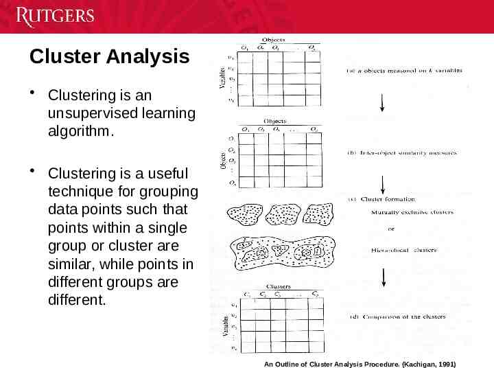
Cluster Analysis Clustering is an unsupervised learning algorithm. Clustering is a useful technique for grouping data points such that points within a single group or cluster are similar, while points in different groups are different. 3 An Outline of Cluster Analysis Procedure. (Kachigan, 1991)

Cluster Analysis: Application Marketing Cluster analysis is used as the methodologies for understanding of the market segments and buyer behaviors. – For example, B. Zafer et al. (2006), Ya-Yueh et al. (2003), Vicki et al. (1992) , Rajendra et al. (1981) , Lewis et al. (2006) , HuaCheng et al. (2005) Market segmentations using cluster analysis have been examined in many different industries. – For instance, finance and banking (Anderson et al, 1976, Calantone et al, 1978), automobile (Kiel et al, 1981), education (Moriarty et al, 1978), consumer product (Sexton, 1974, Schaninger et al, 1980) and high technology industry (Green et al, 1968). 4

Cluster Analysis for Outlier Detection An Outlier is an observation that deviates so much from other observations as to arouse suspicion that it is generated by a different mechanism (Hawkins, 1980) Literatures find outliers as a side-product of clustering algorithms (Ester et al, 1996; Zhang et al, 1996; Wang et al. 1997; Agrawal et al. 1998; Hinneburg and Keim 1998; Guha et al, 1998.) – Distance-based outliers (Knorr and Ng, 1998, 1999; Ramaswamy et al., 2000) – Cluster-based outliers (Knorr and Ng 1999; Jiang et al, 2001, He et al, 2003 ;Duan et al, 2009;) Research Question: How can we apply clustering models for detection of abnormal (fraudulent/erroneous) transactions in continuous auditing? 5

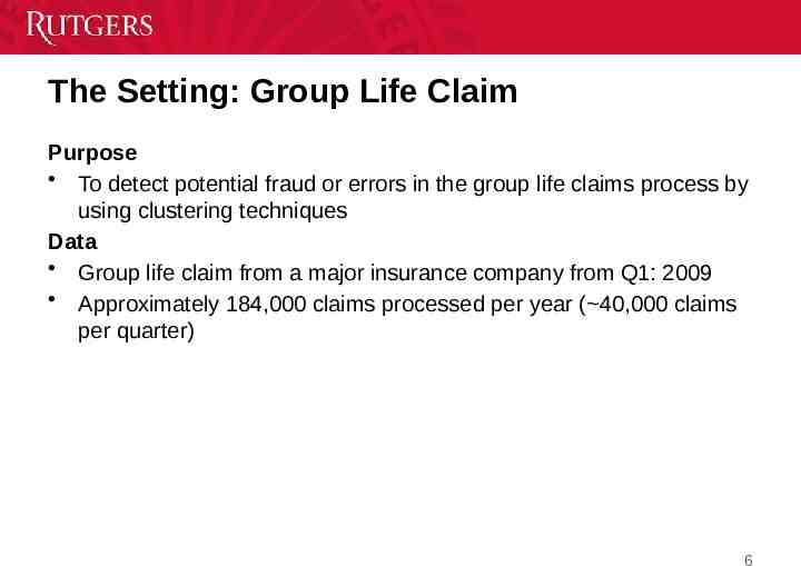
The Setting: Group Life Claim Purpose To detect potential fraud or errors in the group life claims process by using clustering techniques Data Group life claim from a major insurance company from Q1: 2009 Approximately 184,000 claims processed per year ( 40,000 claims per quarter) 6

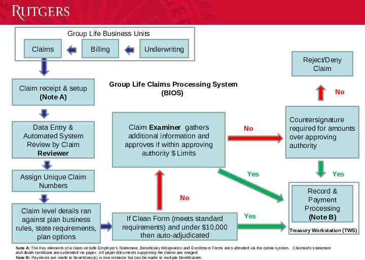
Group Life Business Units Claims Billing Underwriting Reject/Deny Claim Claim receipt & setup (Note A) Data Entry & Automated System Review by Claim Reviewer Group Life Claims Processing System (BIOS) Claim Examiner gathers additional information and approves if within approving authority Limits No No Yes Assign Unique Claim Numbers No Claim level details ran against plan business rules, state requirements, plan options Countersignature required for amounts over approving authority If Clean Form (meets standard requirements) and under 10,000 then auto-adjudicated Yes Yes Record & Payment Processing (Note B) Treasury Workstation (TWS) Note A: The Key elements of a claim include Employer’s Statement, Beneficiary designation and Enrollment Forms are submitted via the online system . Claimant’s statement and death certificate are submitted via paper. All paper documents supporting the claims are imaged. Note B: Payments are made to beneficiary(s) in one instance but can be made to multiple beneficiaries.

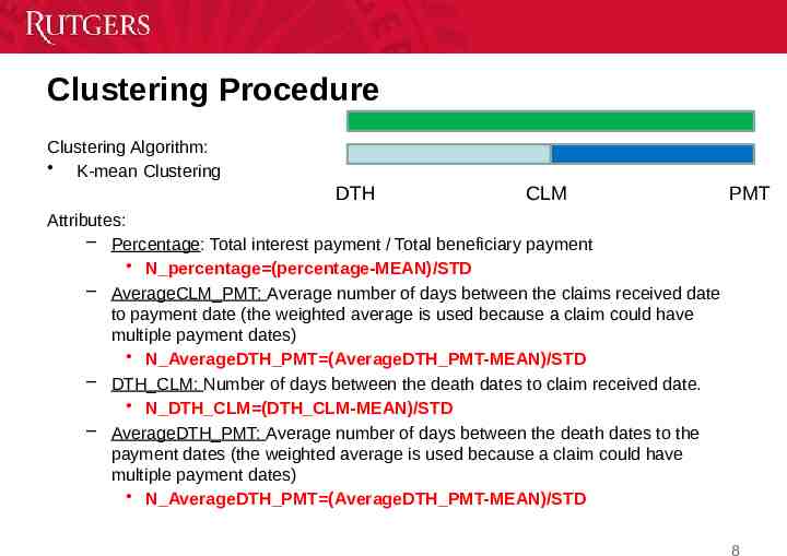
Clustering Procedure Clustering Algorithm: K-mean Clustering DTH CLM PMT Attributes: – Percentage: Total interest payment / Total beneficiary payment N percentage (percentage-MEAN)/STD – AverageCLM PMT: Average number of days between the claims received date to payment date (the weighted average is used because a claim could have multiple payment dates) N AverageDTH PMT (AverageDTH PMT-MEAN)/STD – DTH CLM: Number of days between the death dates to claim received date. N DTH CLM (DTH CLM-MEAN)/STD – AverageDTH PMT: Average number of days between the death dates to the payment dates (the weighted average is used because a claim could have multiple payment dates) N AverageDTH PMT (AverageDTH PMT-MEAN)/STD 8

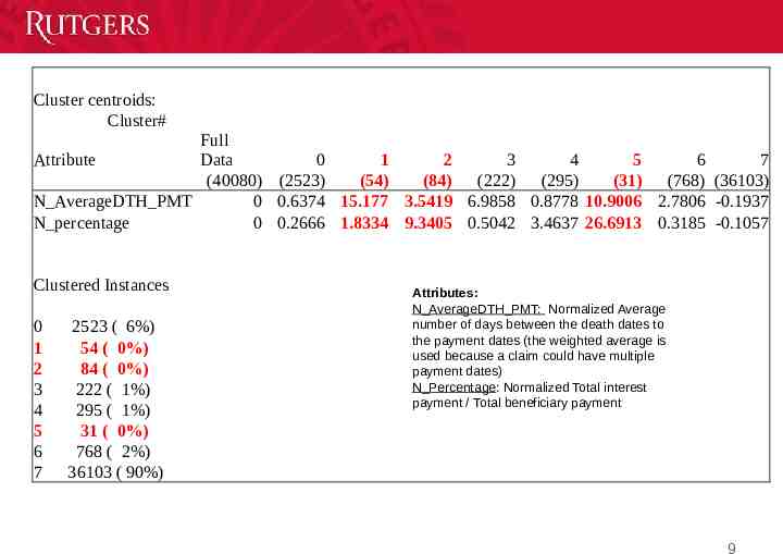
Cluster centroids: Cluster# Full Attribute Data 0 1 2 3 4 5 6 7 (40080) (2523) (54) (84) (222) (295) (31) (768) (36103) N AverageDTH PMT 0 0.6374 15.177 3.5419 6.9858 0.8778 10.9006 2.7806 -0.1937 N percentage 0 0.2666 1.8334 9.3405 0.5042 3.4637 26.6913 0.3185 -0.1057 Clustered Instances 0 1 2 3 4 5 6 7 2523 ( 6%) 54 ( 0%) 84 ( 0%) 222 ( 1%) 295 ( 1%) 31 ( 0%) 768 ( 2%) 36103 ( 90%) Attributes: N AverageDTH PMT: Normalized Average number of days between the death dates to the payment dates (the weighted average is used because a claim could have multiple payment dates) N Percentage: Normalized Total interest payment / Total beneficiary payment 9

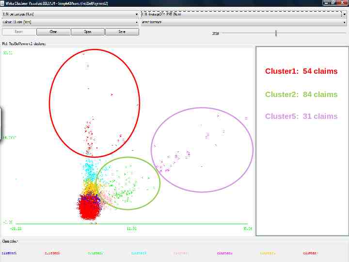
Cluster1: 54 claims Cluster2: 84 claims Cluster5: 31 claims

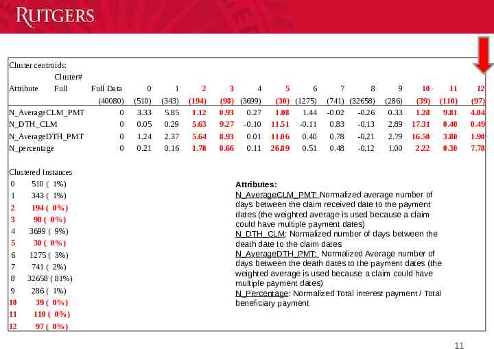
Cluster centroids: Cluster# Attribute Full Full Data (40080) N AverageCLM PMT 0 N DTH CLM 0 N AverageDTH PMT 0 N percentage 0 Clustered Instances 0 510 ( 1%) 1 343 ( 1%) 2 194 ( 0%) 3 98 ( 0%) 4 3699 ( 9%) 5 30 ( 0%) 6 1275 ( 3%) 7 741 ( 2%) 8 32658 ( 81%) 9 286 ( 1%) 10 39 ( 0%) 11 110 ( 0%) 12 97 ( 0%) 0 (510) 3.33 0.05 1.24 0.21 1 (343) 5.85 0.29 2.37 0.16 2 (194) 1.12 5.63 5.64 1.78 3 4 (98) (3699) 0.93 0.27 9.27 -0.10 8.93 0.01 0.66 0.11 5 6 (30) (1275) 1.08 1.44 11.51 -0.11 11.06 0.40 26.89 0.51 7 8 (741) (32658) -0.02 -0.26 0.83 -0.13 0.78 -0.21 0.48 -0.12 9 (286) 0.33 2.89 2.79 1.00 10 (39) 1.28 17.31 16.50 2.22 11 (110) 9.81 0.40 3.80 0.30 Attributes: N AverageCLM PMT: Normalized average number of days between the claim received date to the payment dates (the weighted average is used because a claim could have multiple payment dates) N DTH CLM: Normalized number of days between the death date to the claim dates N AverageDTH PMT: Normalized Average number of days between the death dates to the payment dates (the weighted average is used because a claim could have multiple payment dates) N Percentage: Normalized Total interest payment / Total beneficiary payment 11 12 (97) 4.04 0.49 1.90 7.78

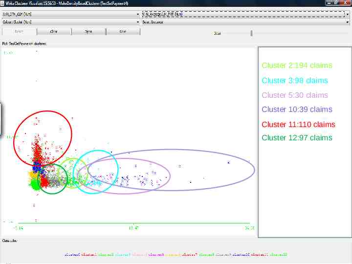
Cluster 2:194 claims Cluster 3:98 claims Cluster 5:30 claims Cluster 10:39 claims Cluster 11:110 claims Cluster 12:97 claims 12

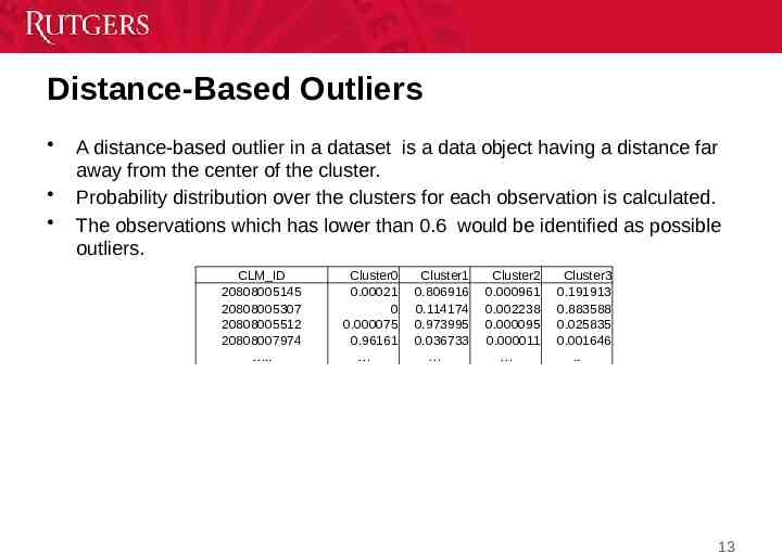
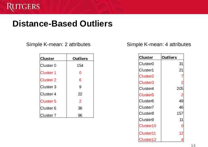
Distance-Based Outliers A distance-based outlier in a dataset is a data object having a distance far away from the center of the cluster. Probability distribution over the clusters for each observation is calculated. The observations which has lower than 0.6 would be identified as possible outliers. CLM ID 20808005145 20808005307 20808005512 20808007974 . Cluster0 0.00021 0 0.000075 0.96161 Cluster1 0.806916 0.114174 0.973995 0.036733 Cluster2 0.000961 0.002238 0.000095 0.000011 Cluster3 0.191913 0.883588 0.025835 0.001646 . 13

Distance-Based Outliers Simple K-mean: 2 attributes Simple K-mean: 4 attributes Cluster Outliers Cluster Outliers Cluster 0 154 Cluster0 31 Cluster 1 0 Cluster1 21 Cluster 2 6 Cluster2 7 Cluster 3 9 Cluster3 2 Cluster4 205 Cluster 4 22 Cluster5 2 Cluster 5 2 Cluster6 49 Cluster 6 36 Cluster7 46 Cluster 7 96 Cluster8 157 Cluster9 11 Cluster10 0 Cluster11 12 Cluster12 4 14

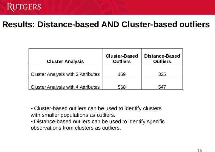
Results: Distance-based AND Cluster-based outliers Cluster Analysis Cluster-Based Outliers Distance-Based Outliers Cluster Analysis with 2 Attributes 169 325 Cluster Analysis with 4 Attributes 568 547 Cluster-based outliers can be used to identify clusters with smaller populations as outliers. Distance-based outliers can be used to identify specific observations from clusters as outliers. 15

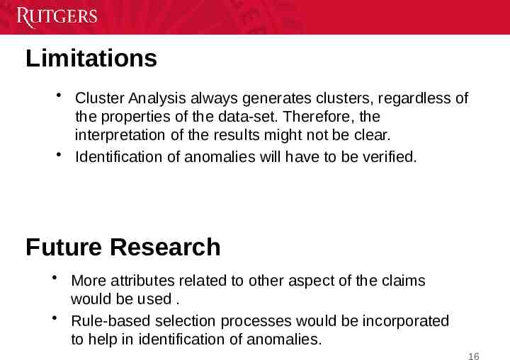
Limitations Cluster Analysis always generates clusters, regardless of the properties of the data-set. Therefore, the interpretation of the results might not be clear. Identification of anomalies will have to be verified. Future Research More attributes related to other aspect of the claims would be used . Rule-based selection processes would be incorporated to help in identification of anomalies. 16