Bivariate Analysis Cross-tabulation and chi-square

Bivariate Analysis Cross-tabulation and chi-square

So far the statistical methods we have used only permit us to: Look at the frequency in which certain numbers or categories occur. Look at measures of central tendency such as means, modes, and medians for one variable. Look at measures of dispersion such as standard deviation and z scores for one interval or ratio level variable.

Bivariate analysis allows us to: Look at associations/relationships among two variables. Look at measures of the strength of the relationship between two variables. Test hypotheses about relationships between two nominal or ordinal level variables.

For example, what does this table tell us about opinions on welfare by gender? Support cutting welfare benefits for immigrants Yes Male Female 15 5 No 10 20 Total 25 25

Are frequencies sufficient to allow us to make comparisons about groups? What other information do we need?

Is this table more helpful? Benefits for Immigrants Males Yes 15 (60%) 5 (20%) No 10 (40%) 20 (80%) Total Female 25 (100%) 25 (100%)

How would you write a sentence or two to describe what is in this table?

Rules for cross-tabulation Calculate either column or row percents. Calculations are the number of frequencies in a cell of a table divided by the total number of frequencies in that column or row, for example 20/25 80.0% All percentages in a column or row should total 100%.

Let’s look at another example – social work degrees by gender Social Work Degree BA Male Female 20 (33.3%) 20 ( %) MSW 30 ( ) 70 (70.0%) Ph.D. 10 (16.7%) 10 (10.0%) 60 (100.0%) 100 (100.0%

Questions: What group had the largest percentage of Ph.Ds? What are the ways in which you could find the missing numbers? Is it obvious why you would use percentages to make comparisons among two or more groups?

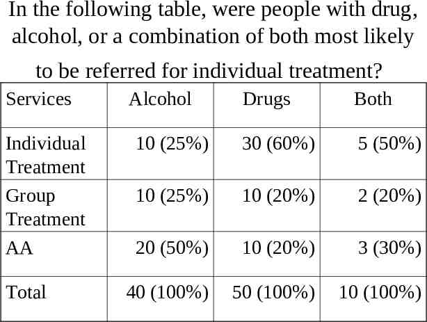
In the following table, were people with drug, alcohol, or a combination of both most likely to be referred for individual treatment? Services Individual Treatment Group Treatment AA Total Alcohol Drugs Both 10 (25%) 30 (60%) 5 (50%) 10 (25%) 10 (20%) 2 (20%) 20 (50%) 10 (20%) 3 (30%) 40 (100%) 50 (100%) 10 (100%)

Use the same table to answer the following question: How much more likely are people with alcohol problems alone to be referred to AA than people with drug problems or a combination of drug and alcohol problems?

We use cross-tabulation when: We want to look at relationships among two or three variables. We want a descriptive statistical measure to tell us whether differences among groups are large enough to indicate some sort of relationship among variables.

Cross-tabs are not sufficient to: Tell us the strength or actually size of the relationships among two or three variables. Test a hypothesis about the relationship between two or three variables. Tell us the direction of the relationship among two or more variables. Look at relationships between one nominal or ordinal variable and one ratio or interval variable unless the range of possible values for the ratio or interval variable is small. What do you think a table with a large number of ratio values would look like?

We can use cross-tabs to visually assess whether independent and dependent variables might be related. In addition, we also use cross-tabs to find out if demographic variables such as gender and ethnicity are related to the second variable.

For example, gender may determine if someone votes Democratic or Republican or if income is high, medium, or low. Ethnicity might be related to where someone lives or attitudes about whether undocumented workers should receive driver’s licenses.

Because we use tables in these ways, we can set up some decision rules about how to use tables. Independent variables should be column variables. If you are not looking at independent and dependent variable relationships, use the variable that can logically be said to influence the other as your column variable. Using this rule, always calculate column percentages rather than row percentages. Use the column percentages to interpret your results.

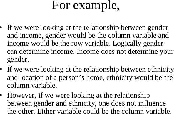
For example, If we were looking at the relationship between gender and income, gender would be the column variable and income would be the row variable. Logically gender can determine income. Income does not determine your gender. If we were looking at the relationship between ethnicity and location of a person’s home, ethnicity would be the column variable. However, if we were looking at the relationship between gender and ethnicity, one does not influence the other. Either variable could be the column variable.

SPSS will allow you to choose a column variable and row variable and whether or not your table will include column or row percents.

You must use an additional statistic, chisquare, if you want to: Test a hypothesis about two variables. Look at the strength of the relationship between an independent and dependent variable. Determine whether the relationship between the two variables is large enough to rule out random chance or sampling error as reasons that there appears to be a relationship between the two variables.

Chi-square is simply an extension of a cross-tabulation that gives you more information about the relationship. However, it provides no information about the direction of the relationship (positive or negative) between the two variables.

Let’s use the following table to test a hypothesis: Education Income High (Above 40,000) High Low Total 40 50 Low ( 39,999 or less) Total 50 50 50 100

I have not filled in all of the information because we need to talk about two concepts before we start calculations: Degrees of Freedom: In any table, there are a limited number of choices for the values in each cell. Marginals: Total frequencies in columns and rows.

Let’s look at the number of choices we have in the previous table: Education Income High (Above 40,000) High Low Total 40 50 Low ( 39,999 or less) Total 50 50 50 100

So the table becomes: Education Income High (Above 40,000) High Low Total 40 10 50 Low ( 39,999 or less) 10 40 50 Total 50 50 100

The rules for determining degrees of freedom in cross-tabulations or contingency tables: In any two by two tables (two columns, two rows, excluding marginals) DF 1. For all other tables, calculate DF as: (c -1 ) * (r-1) where c columns and r rows. ( So for a table with 3 columns and 4 rows, DF . )

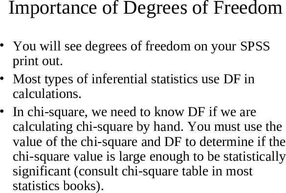
Importance of Degrees of Freedom You will see degrees of freedom on your SPSS print out. Most types of inferential statistics use DF in calculations. In chi-square, we need to know DF if we are calculating chi-square by hand. You must use the value of the chi-square and DF to determine if the chi-square value is large enough to be statistically significant (consult chi-square table in most statistics books).

Steps in testing a hypothesis: State the research hypothesis State the null hypothesis Choose a level of statistical significance (alpha level) Select and compute the test statistic Make a decision regarding whether to accept or reject the null hypothesis.

Calculating Chi-Square Formula is [0 - E]2 E Where 0 is the observed value in a cell E is the expected value in the same cell we would see if there was no association

First steps Alternative hypothesis is: There is a relationship between income level and education for respondents in a survey of BA students. Null hypothesis is: There is no relationship between income level and education for respondents in a survey of BA students Confidence level set at .05

Rules for determining whether the chi-square statistic and probability are large enough to verify a relationship. For hand calculations, use the degree(s) of freedom and the confidence level you set to check the Chi-square table found in most statistics books. For the chi-square to be statistically significant, it must be the same size or larger than the number in the table. On an SPSS print out, the p. or significance value must be the same size or smaller than your significance level.

The formula for expected values are E R*C Education Income High (Above 40,000) High Low Total 25 25 50 Low ( 39,999 or less) 25 25 50 Total 50 50 100

Go back to our first table Education Income High (Above 40,000) High Low Total 40 10 50 Low ( 39,999 or less) 10 40 50 Total 50 50 100

Chi-square calculation is Expected Values Chi-square Cell 1 50 * 50/100 25 (40-25)2/25 9 Cell 2 50*50/100 25 (10-25)2/25 9 Cell 3 50 * 50/100 25 (10-25)2/25 9 Cell 4 50*50/100 25 (40-25)2/25 9 36 At .05, 1 df, chi-square must be larger than 3.84 to be statistically significant

Let’s calculate another chi-square- service receipt by location of residence Service Urban Rural Total Yes 20 40 60 No 30 10 40 Total 50 50 100

For this table, DF 1 Alternative hypothesis: Receiving service is associated with location of residence. Null hypothesis: There is no association between receiving service and location of residence.

Calculations for chi-square are Expected Values Chi-square Cell 1 50 * 60/100 30 (20-30)2/30 3.33 Cell 2 50*40/100 20 (30-20)2/20 5.00 Cell 3 50*60/100 30 (40-30)2/30 3.33 Cell 4 50*40/100 20 (10-20)2/20 5.00 16.67 At 1 DF at .01 chi-square must be greater than 6.64. Do we accept or reject the null hypothesis?

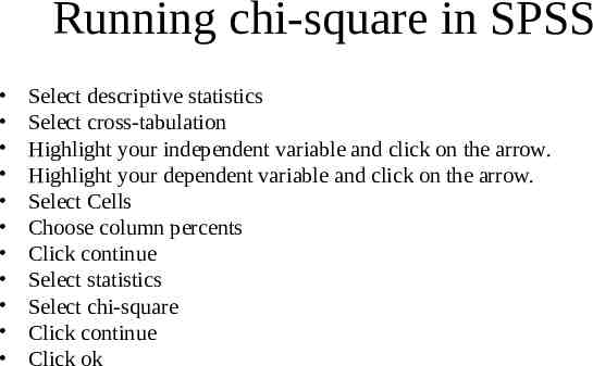
Running chi-square in SPSS Select descriptive statistics Select cross-tabulation Highlight your independent variable and click on the arrow. Highlight your dependent variable and click on the arrow. Select Cells Choose column percents Click continue Select statistics Select chi-square Click continue Click ok

SPSS print out Chi-Square Tests Pearson Chi-Square Likelihood Ratio Linear-by-Linear Association N of Valid Cases Value 2.569a 2.590 .087 5 5 Asymp. Sig. (2-sided) .766 .763 1 .768 df 336 a. 2 cells (16.7%) have expected count less than 5. The minimum expected count is 1.57.

Recode To run ratio or interval level variables into SPSS you need to recode or change the variable into a categorical or nominal or ordinal variable. You first need to decide how you will set up categories and assign a number to them. For example if your ratio variables for Age are: 25, 37, 42, 50, and 64, you might decide on two categories: 1 under 50 2 50 and over

Recode Instructions Go to Transform menu Go to Recode Select different variable Type in new variable name Click continue Enter range of ratio numbers for first category (25 to 49) Enter number for first category (1) in right hand screen. Click Add Enter range of ratio numbers (50 to 54) for category two Enter number for second category (2) Click Add Click Continue Click Change Click o.k.