Assumption MLR.3 Notes (No Perfect Collinearity) Perfect

Assumption MLR.3 Notes (No Perfect Collinearity) Perfect Collinearity can exist if: 1) One variable is a constant multiple of another 2) Logs are used inappropriately 3) One variable is a linear function of two or more other variables In general, all of these issues are easy to fix, once they are identified.

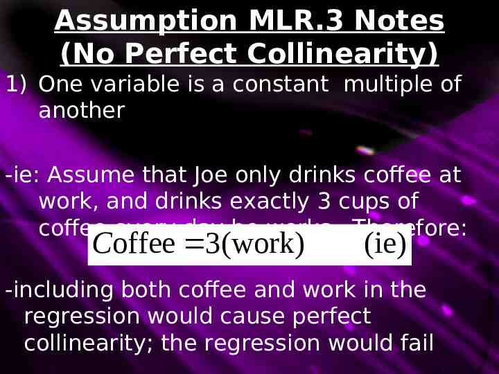
Assumption MLR.3 Notes (No Perfect Collinearity) 1) One variable is a constant multiple of another -ie: Assume that Joe only drinks coffee at work, and drinks exactly 3 cups of coffee every day he works. Therefore: Coffee 3(work) (ie) -including both coffee and work in the regression would cause perfect collinearity; the regression would fail

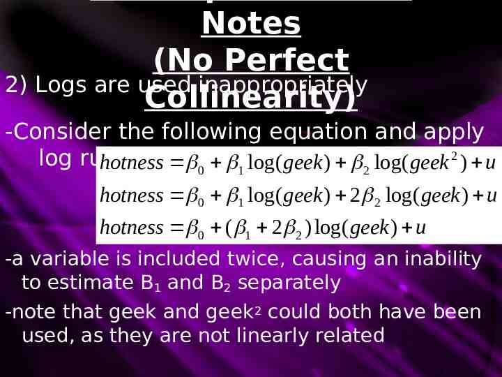
Notes (No Perfect 2) Logs are used inappropriately Collinearity) -Consider the following equation and apply log rules: hotness 0 1 log( geek ) 2 log( geek 2 ) u hotness 0 1 log( geek ) 2 2 log( geek ) u hotness 0 ( 1 2 2 ) log( geek ) u -a variable is included twice, causing an inability to estimate B1 and B2 separately -note that geek and geek2 could both have been used, as they are not linearly related

Notes (No Perfect 3) One variable is a linear function of two Collinearity) or more other variables -Consider a teenager who spends all their income on movies and clothes: income movies clothes -if income and expenditures on both movies and clothes are in the regression, perfect collinearity exists and the regression fails

3.3 Fixing Multicollinearity Drop a variable from the model. If one variable is a multiple of another, it adds nothing to consider it twice Ditto for logs If the elements of a sum are in a regression, the sum itself is redundant. (Alternately one of the elements can be omitted).

3.3 Multicollinearity and N -Assumption MLR.3 can also fail is N is too small -in general, MLR.3 will always fail if n k 1 (the number of parameters) -even if n k 1, MLR.3 may fail due to a bad sample Next we have the most important assumption for proving OLS’s unbiasedness:

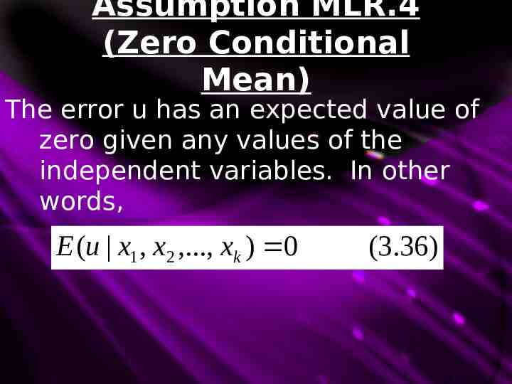
Assumption MLR.4 (Zero Conditional Mean) The error u has an expected value of zero given any values of the independent variables. In other words, E (u x1 , x2 ,., xk ) 0 (3.36)

Assumption MLR.4 Notes (Zero Conditional Mean) MLR.4 fails if the functional relationship is misspecified: 1)A variable is not included the correct way -ie: consumption is included in the regression but not consumption2 and the true relationship is quadratic 2) A variable is included the incorrect way -ie: log(consumption) is included in the regression but consumption is the true relationship -In these cases, the estimators are biased

Assumption MLR.4 Notes (Zero Conditional Mean) MLR.4 also fails if one omits an important factor correlated with any x -this can be due to ignorance or data restrictions MLR.4 also fails due to: 1) Measurement error (ch. 15) 2) An independent variable is jointly determined with y (ch. 16)

Assumption MLR.4 Notes (Zero Conditional Mean) When MLR.4 holds, we have EXOGENOUS EXPLANATORY VARIABLES When MLR.4 does not hold (xj is correlated with u), xj is an ENDOGENOUS EXPLANATORY VARIABLE

MLR.3 vs. MLR.4 (Cage Match) MRL.3 deals with relationships among independent variables -if it fails, OLS cannot run MLR.4 deals with relationships between u and independent variables -it is easier to miss -it is more important

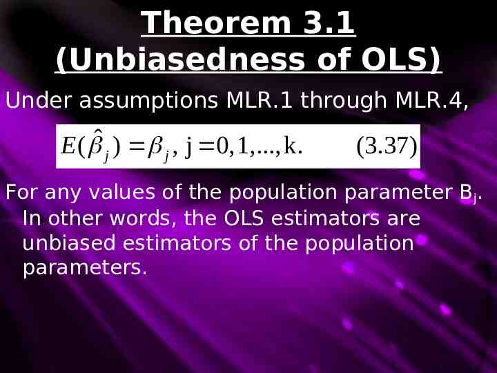
Theorem 3.1 (Unbiasedness of OLS) Under assumptions MLR.1 through MLR.4, E ( ˆ j ) j , j 0, 1,., k. (3.37) For any values of the population parameter Bj. In other words, the OLS estimators are unbiased estimators of the population parameters.

3.3 Is OLS valid? IF OLS runs (B estimates are found) -MLR.3 is satisfied IF the sample is random -MLR.2 is satisfied IF we have some reason to suspect a true relationship -MLR.1 is valid Therefore if we believe MLR.4 holds true -OLS is valid!

3.3 What is unbiasedness? Our estimates of Bhat are all numbers -numbers are fixed, and cannot be biased or unbiased MLR.1 through MLR.4 comments on the OLS PROCEEDURE -Is our assumptions hold true, our OLS PROCEEDURE is unbiased. In other words: “we have no reason to believe our estimate is more likely to be too big or more likely to be too small.”

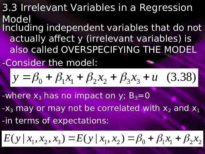
3.3 Irrelevant Variables in a Regression Model Including independent variables that do not actually affect y (irrelevant variables) is also called OVERSPECIFYING THE MODEL -Consider the model: y 0 1 x1 2 x2 3 x3 u (3.38) -where x3 has no impact on y; B3 0 -x3 may or may not be correlated with x2 and x1 -in terms of expectations: E ( y x1 , x2 , x3 ) E ( y x1 , x2 ) 0 1 x1 2 x2

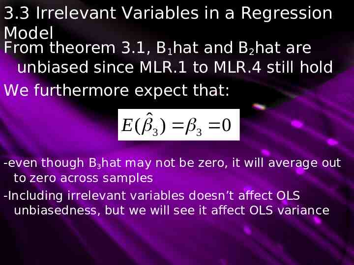
3.3 Irrelevant Variables in a Regression Model From theorem 3.1, B1hat and B2hat are unbiased since MLR.1 to MLR.4 still hold We furthermore expect that: E ( ˆ3 ) 3 0 -even though B3hat may not be zero, it will average out to zero across samples -Including irrelevant variables doesn’t affect OLS unbiasedness, but we will see it affect OLS variance