AP Microeconomics In Class Review #3

AP Microeconomics In Class Review #3

A Producer’s price is derived from 3 things: 1. Cost of Production 2. Competition between firms 3. Demand for product

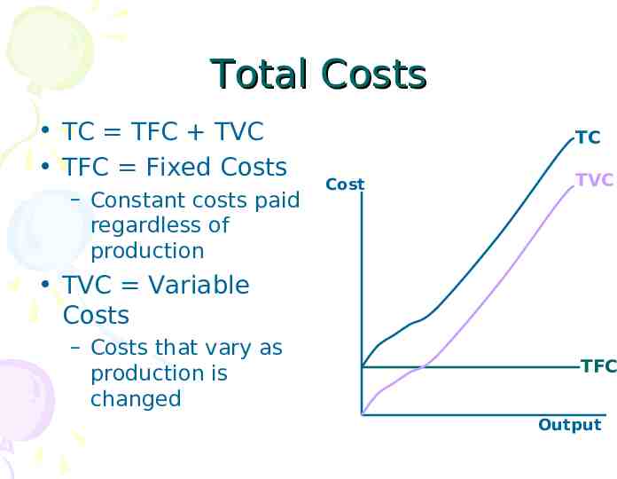
Total Costs TC TFC TVC TFC Fixed Costs – Constant costs paid regardless of production TC Cost TVC TVC Variable Costs – Costs that vary as production is changed TFC Output

Total Revenue TR p q The money received from sale of product Cost & Revenue TC TR Break Even Profit Loss Output

Profit TR - TC Accounting: Calculates actual costs a business incurs Explicit!! Ex) inputs, salaries, rent, both fixed and variable Economic: Calculates all accounting costs plus the what if, or opportunity, costs Implicit!!!! Ex) what was given up, lost interest, “freebie” costs

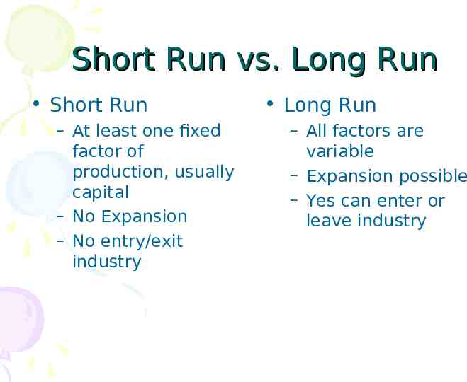
Short Run vs. Long Run Short Run – At least one fixed factor of production, usually capital – No Expansion – No entry/exit industry Long Run – All factors are variable – Expansion possible – Yes can enter or leave industry

Production Considerations Total Product: the relationship btwn inputs and outputs Marginal Product: the extra product gained by the change in inputs; MP ΔTP Average Product: AP TP/q

The Production Function Input Total Product 1 10 2 24 3 39 4 52 5 60 6 66 7 63 8 56 Marginal Product Average Product 10 14 15 13 8 6 -3 -7 10 12 13 13 12 11 9 7 Stages of Production I I I II II II III III

Key Graph Parts to Remember: Stages follow MP AP intersects MP at its high point MP increases, decrease & then goes negative Output TP AP MP

Production Function 8. Law of Diminishing Returns Due to limited capacity, output will slow down and then decrease beyond a certain point 9. Choice of Technology Capital (K) and Labor (L) are both complements and substitutes, firms will find the combination that is the most efficient (cheapest)

Producer’s Costs TFC: Total Fixed Costs AFC: Average Fixed Costs; TFC/q AVC: Average Variable Costs; TVC/q Marginal Costs ΔTC

Perfect Competition Characteristics: many firms, homogenous products, no barriers to entry, P MC MR Marginal Revenue: extra revenue gained with each additional unit of output; MR ΔTR P d MR: Price Takers, each firm takes market price (or market demand) so P and MR are constant (perfectly elastic & horizontal)

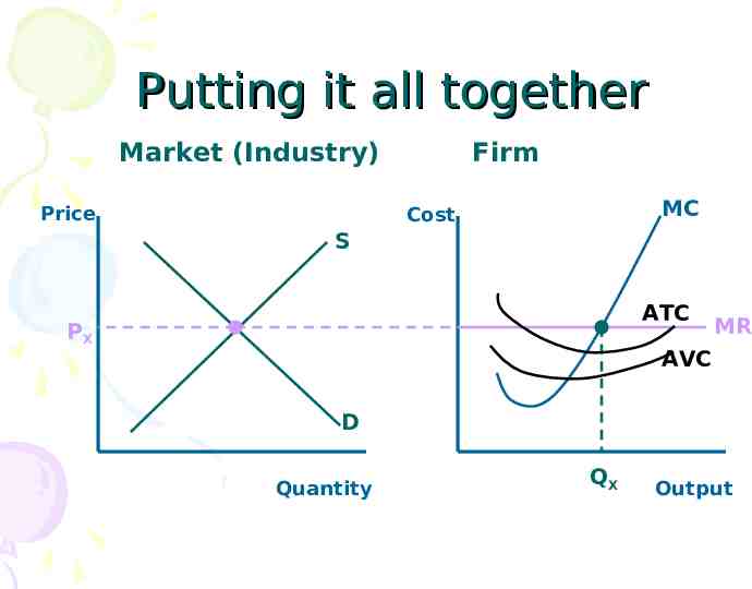
Putting it all together Market (Industry) Price Firm MC Cost S ATC PX MR AVC D Quantity QX Output

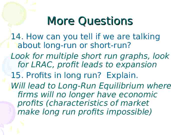
More Questions 14. How can you tell if we are talking about long-run or short-run? Look for multiple short run graphs, look for LRAC, profit leads to expansion 15. Profits in long run? Explain. Will lead to Long-Run Equilibrium where firms will no longer have economic profits (characteristics of market make long run profits impossible)

GRAPH: LRAC Price Market S0 Cost S1 Firm SRMC P0 SRMC SRAC SRAC LRAC P1 D Quantity Level #1 Level #2 Outputs

Operating Profit: Minimizing losses, it is better to produce and lose a little than it is to produce nothing and lose total fixed costs TR - TVC Choices: produce with loss Cost MC ATC PX Losses MR AVC Op. Profit QX Output

Shutting Down vs. Exiting the Industry Shutting Down: Short Run option Still paying out Total Fixed Costs but not producing Exiting: Long Run option No costs, no production, business no longer exists

Expanding Production Economies of Scale – LR, expand and more efficient (decrease costs) Diseconomies of Scale – LR, expand and less efficient (increase costs) Constant Return to Scale – LR, expand and costs are same per unit

Expanding Production Increasing Returns – LR, expand and increase production Diminishing Returns – LR, expand and decrease production

Graphing Expansion Firm Constant returns to scale Diseconomies of scale Unit Costs Economies of scale Long-run ATC Output

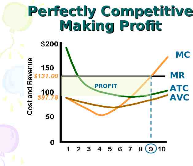
Perfectly Competitive Making Profit MC PROFIT MR ATC AVC

Perfectly Competitive Minimizing Losses Any Price btwn the average cost curves represents an economic loss but an operating profit

Perfectly Competitive Breaking Even

Perfectly Competitive Shut Down Any Price below AVC’s min point represent total loss

Derived Demand: the demand for labor is directly dependent on the demand for the output that labor creates Law of Diminishing Returns & Hiring Labor: there is a limit to how many workers a firm should hire (SR), hire as long as they are efficient

Income vs. Substitution Substitution Effect Choose to subs work for leisure to get more money Income Effect Choose current income with less work, want more leisure time Normal Supply Curve Backward Bending PL PL SL SL QL QL

Marginal Product of Labor: (MPL) The additional output produced as one more unit of labor is added Marginal Revenue Product of Labor: (MRPL) The addition to the firm’s revenue as the result of the marginal product per labor unit – Represents the firm’s demand curve for labor

Marginal Resource Cost Wage of Labor Price of Labor MRC WL PL All refer to the cost of the input labor and are interchangeable. In a perfectly competitive labor market, the PL comes from market and is a horizontal line for the firm – It is the supply curve of labor faced by the firm

Example: PL 60 and PX 10 Labor (L) Total Output (Q) 1 2 3 4 5 5 20 30 35 35 MPL ΔOutput Marginal Product (MPL) 5 15 10 5 0 Marginal Revenue Product (MRPL) 50 150 100 50 0 MRPL MPL PX

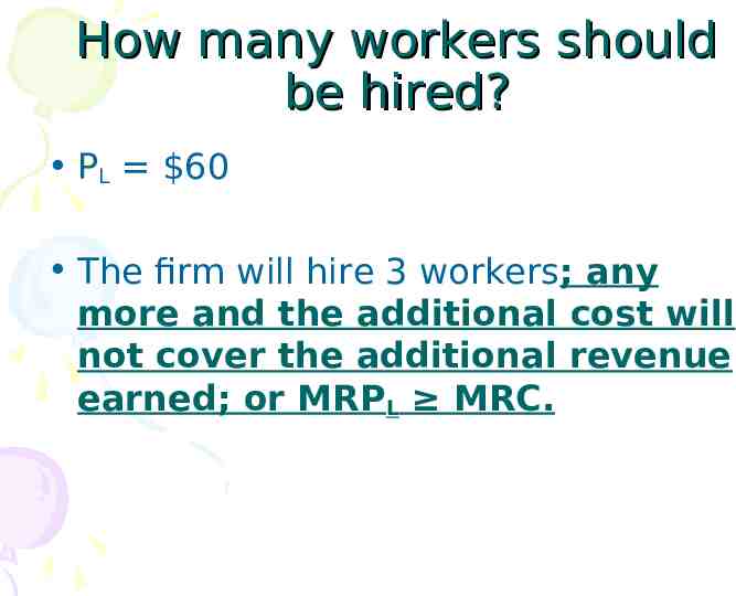
How many workers should be hired? PL 60 The firm will hire 3 workers; any more and the additional cost will not cover the additional revenue earned; or MRPL MRC.

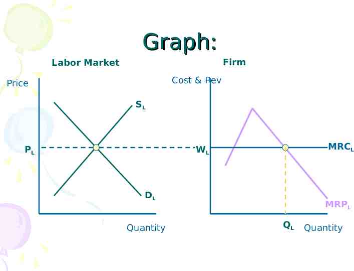
Graph: Firm Labor Market Cost & Rev Price SL PL MRCL WL DL Quantity MRPL QL Quantity

Parts to Remember: #1: MRC is the labor supply curve available to the firm #2: MRP is the labor demand curve of the firm #3: find where they intersect and that is the quantity of labor hired!! (MC MR)