Advanced Thermodynamics Note 10 Solution Thermodynamics: Theory

Advanced Thermodynamics Note 10 Solution Thermodynamics: Theory Lecturer: 郭修伯

Compositions Real system usually contains a mixture of fluid. Develop the theoretical foundation for applications of thermodynamics to gas mixtures and liquid solutions Introducing – – – – – chemical potential partial properties fugacity excess properties ideal solution

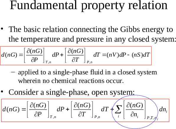
Fundamental property relation The basic relation connecting the Gibbs energy to the temperature and pressure in any closed system: (nG) (nG) d (nG) dP dT (nV )dP (nS )dT P T ,n T P ,n – applied to a single-phase fluid in a closed system wherein no chemical reactions occur. Consider a single-phase, open system: (nG ) (nG ) (nG ) d (nG ) dP dT dni P T ,n T P ,n i ni P ,T , n j

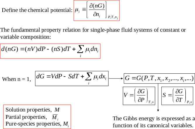
(nG ) Define the chemical potential: i n i P ,T , n j The fundamental property relation for single-phase fluid systems of constant or variable composition: d (nG ) (nV )dP (nS )dT i dni i When n 1, dG VdP SdT dx i i i G G ( P, T , x1 , x2 ,., xi ,.) G V P T ,x Solution properties, M Partial properties, M i Pure-species properties, Mi G S T P,x The Gibbs energy is expressed as a function of its canonical variables.

Chemical potential and phase equilibria Consider a closed system consisting of two phases in equilibrium: d (nG ) (nV ) dP (nS ) dT i dni d (nG ) (nV ) dP (nS ) dT i dni i i nM (nM ) (nM ) d (nG ) (nV )dP (nS )dT i dni i dni i Multiple phases at the same T and P are in equilibrium when chemical potential of each species is the same in all phases. i Mass balance: dni dni i i

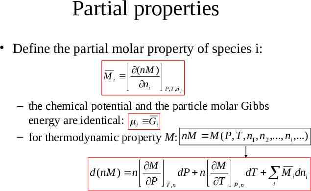
Partial properties Define the partial molar property of species i: (nM ) M i n i P ,T ,n j – the chemical potential and the particle molar Gibbs energy are identical: i Gi – for thermodynamic property M: nM M ( P, T , n1 , n2 ,., ni ,.) M M d (nM ) n dP n dT M i dni P T , n T P ,n i

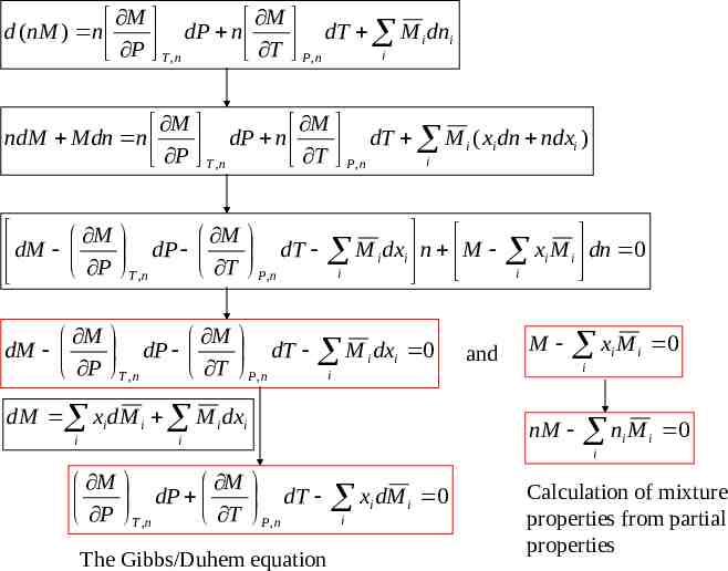
M M d (nM ) n dP n dT M i dni P T ,n T P ,n i M M ndM Mdn n dP n dT M i ( xi dn ndxi ) P T ,n T P ,n i M M dM dP dT P T ,n T P ,n M M dM dP dT P T ,n T P ,n M dx n i i i M M dx i i 0 The Gibbs/Duhem equation xM i i 0 i nM i M M dP dT P T ,n T P ,n M i dM xi dM i M i dxi i and x M i i i dn 0 n M i i 0 i x dM i i i 0 Calculation of mixture properties from partial properties

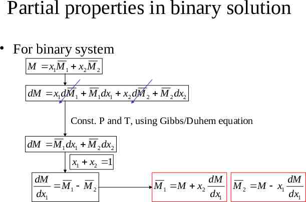
Partial properties in binary solution For binary system M x1M 1 x2 M 2 dM x1dM 1 M 1dx1 x2 dM 2 M 2 dx2 Const. P and T, using Gibbs/Duhem equation dM M 1dx1 M 2 dx2 x1 x2 1 dM M 1 M 2 dx1 M 1 M x 2 dM dx1 M 2 M x1 dM dx1

The need arises in a laboratory for 2000 cm3 of an antifreeze solution consisting of 30 mol-% methanol in water. What volumes of pure methanol and of pure water at 25 C must be mixed to form the 2000 cm3 of antifreeze at 25 C? The partial and pure molar volumes are given. V x1V1 x2V2 V (0.3)(38.632) (0.7)(17.765) 24.025 cm3 / mol Vt 2000 n 83.246 mol V 24.025 n1 (0.3)(83.246) 24.974 mol n2 (0.7)(83.246) 58.272 mol V1t n1V1 (24.974)(40.727) 1017 cm3 V2t n2V2 (58.272)(18.068) 1053 cm3 Fig 11.2

Fig 11.2

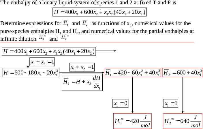
The enthalpy of a binary liquid system of species 1 and 2 at fixed T and P is: H 400 x1 600 x2 x1 x2 (40 x1 20 x2 ) Determine expressions for H1 and H 2 as functions of x1, numerical values for the pure-species enthalpies H1 and H2, and numerical values for the partial enthalpies at H H 1 2 infinite dilution and H 400 x1 600 x2 x1 x2 (40 x1 20 x2 ) x1 x2 1 3 1 H 600 180 x1 20 x x1 x2 1 H 1 H x2 dH dx1 H1 420 60 x12 40 x13 H 2 600 40 x13 x1 0 H1 420 x1 1 J mol H 2 640 J mol

Relations among partial properties d (nG ) (nV )dP (nS )dT Gi dni i Maxwell relation: V S T P ,n P T ,n Gi T (nS ) n P ,n i P ,T , n j Gi T S i P ,x Gi P (nV ) n T ,n i P ,T , n j Gi P dGi Vi dP S i dT H U PV H i U i PVi Vi T ,x

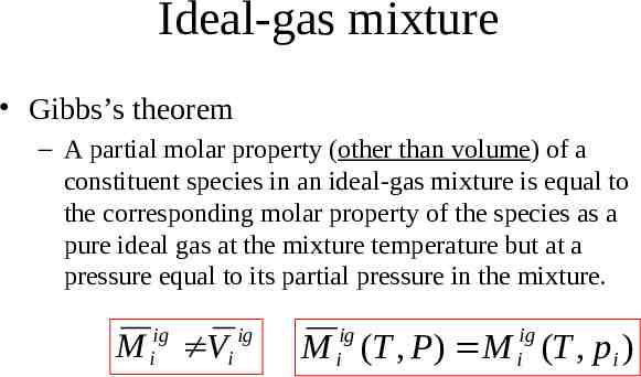
Ideal-gas mixture Gibbs’s theorem – A partial molar property (other than volume) of a constituent species in an ideal-gas mixture is equal to the corresponding molar property of the species as a pure ideal gas at the mixture temperature but at a pressure equal to its partial pressure in the mixture. M iig Vi ig ig i ig i M (T , P ) M (T , pi )

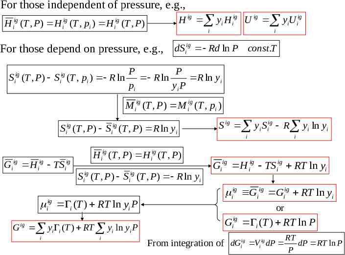
For those independent of pressure, e.g., ig i ig i H ig yi H iig U ig yiU iig ig i H (T , P ) H (T , pi ) H (T , P) i i For those depend on pressure, e.g., dSiig Rd ln P const.T Siig (T , P ) S iig (T , pi ) R ln P P R ln R ln yi pi yi P M iig (T , P ) M iig (T , pi ) ig i ig i S (T , P) S (T , P ) R ln yi Gi ig H iig TSiig H iig (T , P) H iig (T , P ) S iig (T , P) S iig (T , P) R ln yi iig i (T ) RT ln yi P ig G yi i (T ) RT yi ln yi P i i S ig yi Siig R yi ln yi i i Gi ig H iig TS iig RT ln yi iig Gi ig Giig RT ln yi or Giig i (T ) RT ln P From integration of dGiig Vi ig dP RT dP RT ln P P

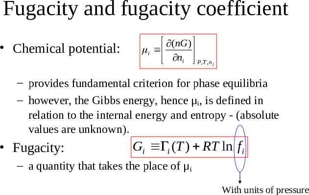
Fugacity and fugacity coefficient Chemical potential: (nG ) i n i P ,T , n j – provides fundamental criterion for phase equilibria – however, the Gibbs energy, hence μi, is defined in relation to the internal energy and entropy - (absolute values are unknown). Fugacity: Gi i (T ) RT ln f i – a quantity that takes the place of μi With units of pressure

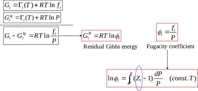
Gi i (T ) RT ln f i Giig i (T ) RT ln P fi ig Gi Gi RT ln P fi i P GiR RT ln i Residual Gibbs energy Fugacity coefficient dP ln i ( Z i 1) 0 P P (const. T )

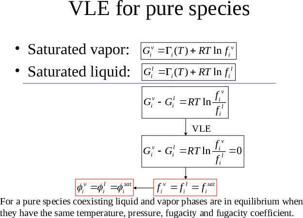
VLE for pure species Saturated vapor: Saturated liquid: Giv i (T ) RT ln f i v Gil i (T ) RT ln f i l fi v G G RT ln l fi v i l i VLE v f Giv Gil RT ln i l 0 fi iv il isat f i v f i l f i sat For a pure species coexisting liquid and vapor phases are in equilibrium when they have the same temperature, pressure, fugacity and fugacity coefficient.

Fugacity of a pure liquid The fugacity of pure species i as a compressed liquid: Gi Gisat RT ln ln fi fi sat 1 RT fi f i sat P Pi sat sat i Gi G P sat Vi dP (isothermal process ) Pi Vi dP Since Vi is a weak function of P ln fi f i sat Vi l ( P Pi sat ) RT fi sat sat sat i i P sat sat i i f i P Vi l ( P Pi sat ) exp RT

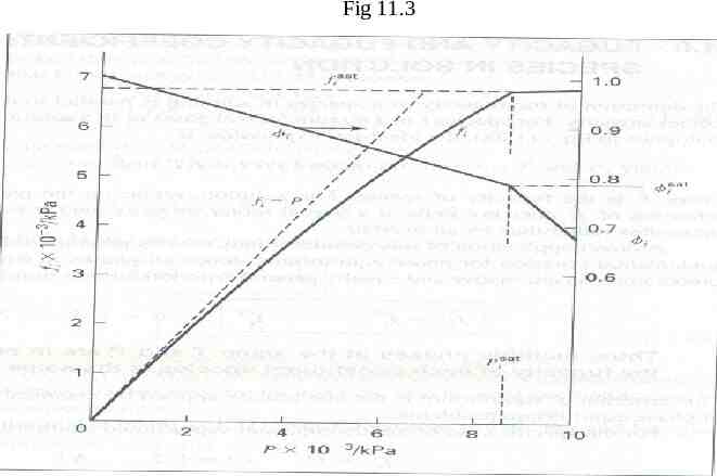
For H2O at a temperature of 300 C and for pressures up to 10,000 kPa (100 bar) calculate values of fi and φi from data in the steam tables and plot them vs. P. For a state at P: Gi i (T ) RT ln f i For a low pressure reference state: Gi* i (T ) RT ln f i * fi 1 * fi 1 H i H i* * ln ( G G ) i i ln * ( Si Si ) * fi RT fi R T Gi H i TS i The low pressure (say 1 kPa) at 300 C: f i* P * 1 kPa S * 10.3450 J i gK H i* 3076.8 J g For different values of P up to the saturated pressure at 300 C, one obtains the values of fi ,and hence φi . Note, values of fi and φi at 8592.7 kPa are obtained Values of fi andφi at higher pressure: sat sat i i f i P Fig 11.3 Vi l ( P Pi sat ) exp RT

Fig 11.3

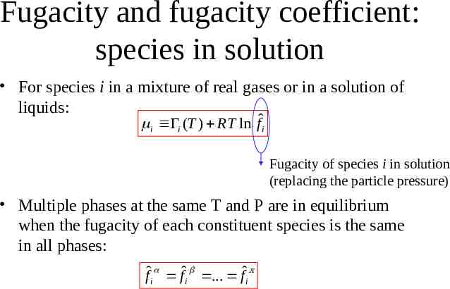
Fugacity and fugacity coefficient: species in solution For species i in a mixture of real gases or in a solution of liquids: i i (T ) RT ln fˆi Fugacity of species i in solution (replacing the particle pressure) Multiple phases at the same T and P are in equilibrium when the fugacity of each constituent species is the same in all phases: fˆi fˆi . fˆi

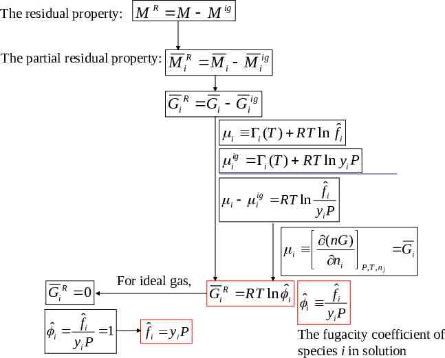
The residual property: M R M M ig The partial residual property: M R M M ig i i i Gi R Gi Gi ig i i (T ) RT ln fˆi iig i (T ) RT ln yi P fˆi i RT ln yi P ig i R Gi 0 fˆi ˆ i 1 yi P For ideal gas, fˆi yi P (nG ) i Gi ni P ,T ,n j fˆi Gi R RT ln ˆi ˆ i yi P The fugacity coefficient of species i in solution

Fundamental residual-property relation 1 nG nG d d (nG ) dT 2 RT RT RT d (nG ) (nV )dP (nS )dT i dni i G H TS Gi nH nG nV d dP dT dni 2 RT RT RT i RT nG f ( P, T , ni ) RT G/RT as a function of its canonical variables allows evaluation of all other thermodynamic properties, and implicitly contains complete property information. The residual properties: R nG R nV R nH R Gi d dP dT dni 2 RT i RT RT RT nG R or d RT nV R nH R dP dT ln ˆi dni 2 RT i RT

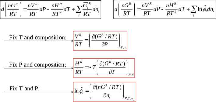
R nG R nV R Gi nH R d dP dT dni 2 RT i RT RT RT nG R d RT nV R nH R dP dT ln ˆi dni 2 RT i RT Fix T and composition: V R (G R / RT ) RT P T ,x Fix P and composition: (G R / RT ) HR T RT T P,x Fix T and P: R ( nG / RT ) ln ˆi n i P ,T ,n j

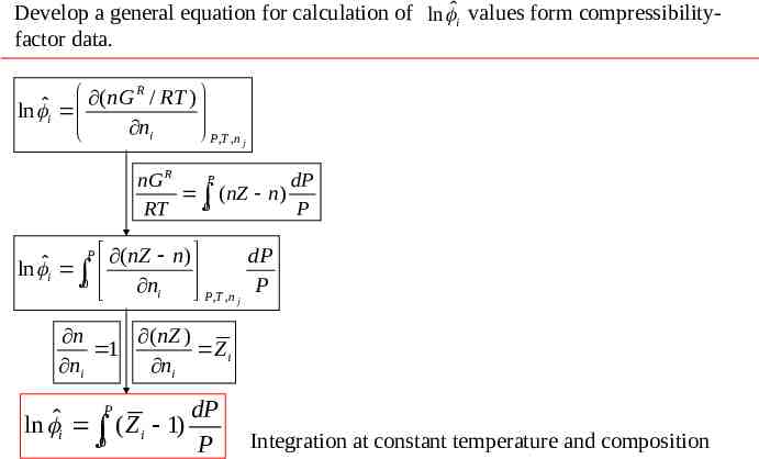
Develop a general equation for calculation of ln ˆi values form compressibilityfactor data. R ( nG / RT ) ln ˆi ni P ,T ,n j P nG R dP (nZ n) 0 RT P P ( nZ n) dP ˆ ln i 0 n i P ,T ,n j P n (nZ ) 1 Z i ni ni P dP ˆ ln i ( Z i 1) 0 P Integration at constant temperature and composition

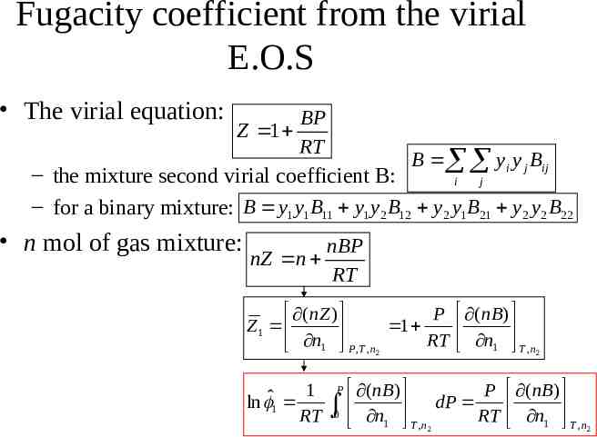
Fugacity coefficient from the virial E.O.S The virial equation: BP Z 1 RT B yi y j Bij – the mixture second virial coefficient B: i j – for a binary mixture: B y1 y1 B11 y1 y2 B12 y2 y1 B21 y2 y2 B22 n mol of gas mixture: nBP nZ n RT (nZ ) P Z1 1 n RT 1 P ,T , n2 1 ln ˆ1 RT (nB) n 1 T , n2 (nB) P dP 0 n1 RT T , n2 P (nB) n 1 T , n2

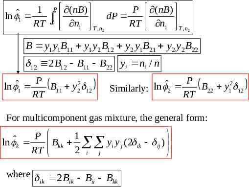
1 ln ˆ1 RT (nB) P (nB) dP 0 n1 RT n 1 T , n2 T , n2 P B y1 y1 B11 y1 y2 B12 y2 y1 B21 y2 y2 B22 12 2 B12 B11 B22 yi ni / n P ˆ ln 1 B11 y22 12 RT P ˆ B22 y12 12 Similarly: ln 2 RT For multicomponent gas mixture, the general form: P 1 ˆ ln k Bkk yi y j (2 ik ij ) RT 2 i j where 2 B B B ik ik ii kk

Determine the fugacity coefficients for nitrogen and methane in N2(1)/CH4(2) mixture at 200K and 30 bar if the mixture contains 40 mol-% N2. 3 12 2 B12 B11 B22 2( 59.8) 35.2 105.0 20.6 cm mol P 30 ln ˆ1 B11 y22 12 35.2 (0.6) 2 (20.6) 0.0501 RT (83.14)(200) ˆ1 0.9511 P 30 2 ˆ ln 2 B22 y1 12 105.0 (0.4) 2 (20.6) 0.1835 RT (83.14)(200) ˆ2 0.8324

Generalized correlations for the fugacity coefficient dPr ln i ( Z i 1) 0 Pr Pr Z 1 (const. Tr ) Pr 0 ( B B 1 ) Tr Z Z 0 Z 1 Pr dP dP ln ( Z 1) r Z 1 r 0 0 Pr Pr Pr 0 PHIB(TR, PR, OMEGA) (const. Tr ) or ln ln 0 ln 1 with Pr dPr dP 1 ln ( Z 1) ln Z 1 r For pure gas 0 0 Pr Pr 0 Pr 0 Table E1:E4 or Pr 0 ln ( B B1 ) Tr Table E13:E16 For pure gas

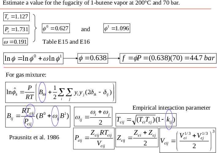
Estimate a value for the fugacity of 1-butene vapor at 200 C and 70 bar. Tr 1.127 Pr 1.731 0 0.627 0.191 Table E15 and E16 ln ln 0 ln 1 and 1 1.096 0.638 f P (0.638)(70) 44.7 bar For gas mixture: P 1 ˆ Bkk yi y j (2 ik ij ) ln k RT 2 i j Bij RTcij Pcij Empirical interaction parameter i j Tcij (TciTcj ) (1 kij ) 2 1/ 3 1/ 3 3 Z ci Z cj Z cij RTcij Vci Vcj Pcij Z cij Vcij Vcij 2 2 ( B 0 ij B1 ) ij Prausnitz et al. 1986

ˆ ˆ Estimate 1 and 2 for an equimolar mixture of methyl ethyl ketone (1) / toluene (2) at 50 C and 25 kPa. Set all kij 0. 1/ 3 1/ 3 3 i j Z ci Z cj Z cij RTcij Vci Vcj ij Z cij Pcij Vcij 2 2 Vcij 2 RTcij 0 Tcij (TciTcj ) (1 kij ) 12 2 B12 B11 B22 1 Bij ( B ij B ) Pcij P ln ˆ1 B11 y22 12 0.0128 RT ˆ1 0.987 P ln ˆ2 B22 y12 12 0.0172 RT ˆ2 0.983

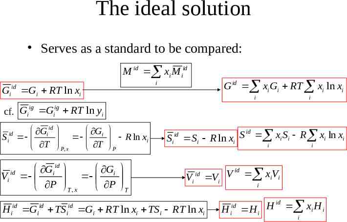
The ideal solution Serves as a standard to be compared: M id xi M iid G id xi Gi RT xi ln xi i id Gi Gi RT ln xi i i ig ig cf. Gi Gi RT ln yi S id i Gi id T Vi id H id i G i P,x T Gi id P id R ln xi P G i T ,x P Gi TS id i T S id i id S xi S i R xi ln xi Si R ln xi i Vi id i id V xiVi Vi Gi RT ln xi TSi RT ln xi i H id i id H xi H i H i i

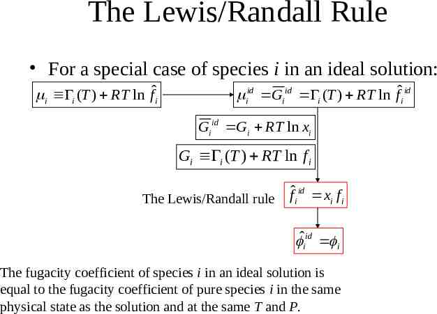
The Lewis/Randall Rule For a special case of species i in an ideal solution: i i (T ) RT ln fˆi iid Gi id i (T ) RT ln fˆi id Gi id Gi RT ln xi Gi i (T ) RT ln f i The Lewis/Randall rule fˆi id xi f i ˆiid i The fugacity coefficient of species i in an ideal solution is equal to the fugacity coefficient of pure species i in the same physical state as the solution and at the same T and P.

Excess properties The mathematical formalism of excess properties is analogous to that of the residual properties: M E M M id – where M represents the molar (or unit-mass) value of any extensive thermodynamic property (e.g., V, U, H, S, G, etc.) – Similarly, we have: nG E d RT E nV E Gi nH E dP dT dni 2 RT i RT RT The fundamental excess-property relation

Table 11.1

(1) If CEP is a constant, independent of T, find expression for GE, SE, and HE as functions of T. (2) From the equations developed in part (1), fine values for G E , SE, and HE for an equilmolar solution of benzene(1) / n-hexane(2) at 323.15K, given the following excess-property values for equilmolar solution at 298.15K: CEP -2.86 J/mol-K, HE 897.9 J/mol, and GE 384.5 J/mol 2G E From Table 11.1: C T 2 T E P P , x C PE a const. 2G E 2 T a T P,x integration G E From Table 11.1: S T E P,x integration S E a ln T b G E T a ln T b P,x integration G E a (T ln T T ) bT c H E G E TS E aT c C PE a 2.86 897.9 a (298.15) c 384.5 a((298.15) ln(298.15) (298.15) b(198.15) c We have values of a, b, c and hence the excessproperties at 323.15K

The excess Gibbs energy and the activity coefficient The excess Gibbs energy is of particular interest: G E G G id Gi i (T ) RT ln fˆi Gi id i (T ) RT ln xi f i fˆi Gi RT ln xi f i E fˆi i xi f i Gi E RT ln i c.f. Gi R RT ln ˆi The activity coefficient of species i in solution. A factor introduced into Raoult’s law to account for liquid-phase non-idealities. For ideal solution, Gi E 0, i 1

nG E d RT E nV E Gi nH E dP dT dni 2 RT RT RT i nG E d RT nV E nH E dP dT ln i dni 2 RT RT i V E (G E / RT ) RT P T ,x E E (G / RT ) H T RT T P,x Experimental accessible values: activity coefficients from VLE data, VE and HE values come from mixing experiments. (nG E / RT ) ln i ni P ,T ,n j GE xi ln i RT i x d ln i i i 0 (const. T , P ) Important application in phase-equilibrium thermodynamics.

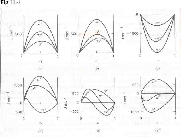
The nature of excess properties GE: through reduction of VLE data HE: from mixing experiment SE (HE - GE) / T Fig 11.4 – excess properties become zero as either species 1. – GE is approximately parabolic in shape; H E and TSE exhibit individual composition dependence. – The extreme value of ME often occurs near the equilmolar composition.

Fig 11.4