291K Machine Learning Unsupervised Learning Lei Li and Yu-xiang Wang

291K Machine Learning Unsupervised Learning Lei Li and Yu-xiang Wang UCSB Some slides borrowed from Eric Xing, Arti Singh 1

Recap Linear Regression Linear classifier Both need pairs of data-labels x, y to train What if we do not have labels y – Can we still train a model to predict data class? 2

Unsupervised Learning Basically finding “patterns” of data No golden labels to teach the model – Only raw data x, but not y Instances: – Clustering: Give data samples, find groupings – Dimensionality Reduction: Given highdimensional data, compress them into lowdimensions 3

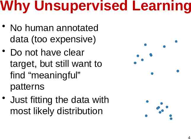
Why Unsupervised Learning No human annotated data (too expensive) Do not have clear target, but still want to find “meaningful” patterns Just fitting the data with most likely distribution 4

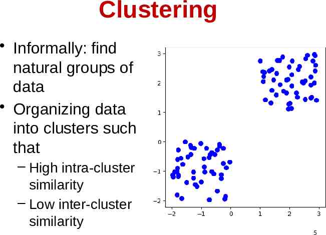
Clustering Informally: find natural groups of data Organizing data into clusters such that – High intra-cluster similarity – Low inter-cluster similarity 5

Grouping News Articles Benjamin Netanyahu Questioned in Israel Graft Inquiry Rockefeller Foundation Picks Rajiv J. Shah, a Trustee, as President lare Hollingworth, Reporter Who Broke News of World War II, Dies at 105 Danielle Brooks: The First Time I Saw Myself on a Billboard For Troubled Student, a Change of School and Direction 10 Key Moments and More From Trump’s News Conference California Today: The Tale of the Laguna Beach Jumper 6

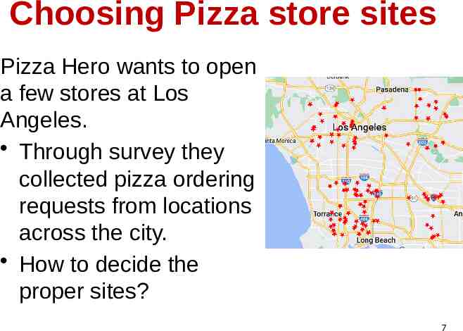
Choosing Pizza store sites Pizza Hero wants to open a few stores at Los Angeles. Through survey they collected pizza ordering requests from locations across the city. How to decide the proper sites? 7

Why Clustering? Organizing data into clusters provides better interpretation of the data – Reveal internal structure of data samples Partition the data itself can be the goal – Image segmentation: separating objects from background Knowledge discovery in data – E.g. reoccurring patterns, topics, etc. 8

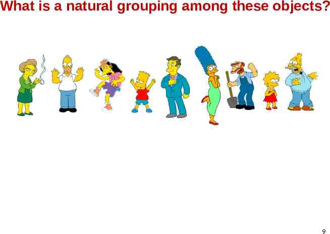
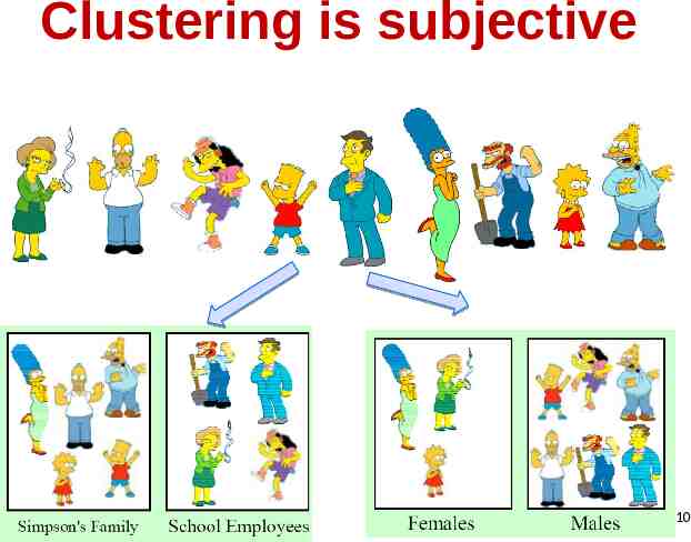
What is a natural grouping among these objects? 9

Clustering is subjective 10

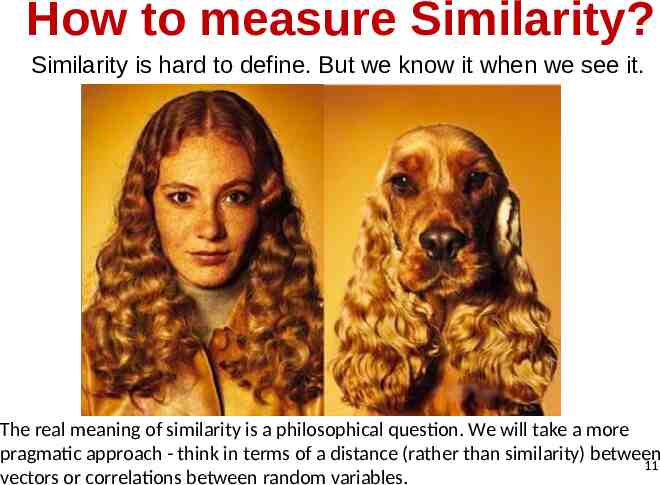
How to measure Similarity? Similarity is hard to define. But we know it when we see it. The real meaning of similarity is a philosophical question. We will take a more pragmatic approach - think in terms of a distance (rather than similarity) between 11 vectors or correlations between random variables.

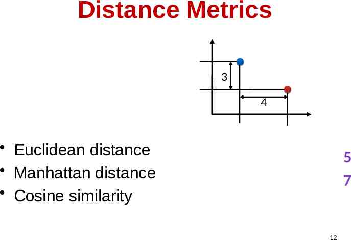
Distance Metrics 3 4 Euclidean distance Manhattan distance Cosine similarity 5 7 12

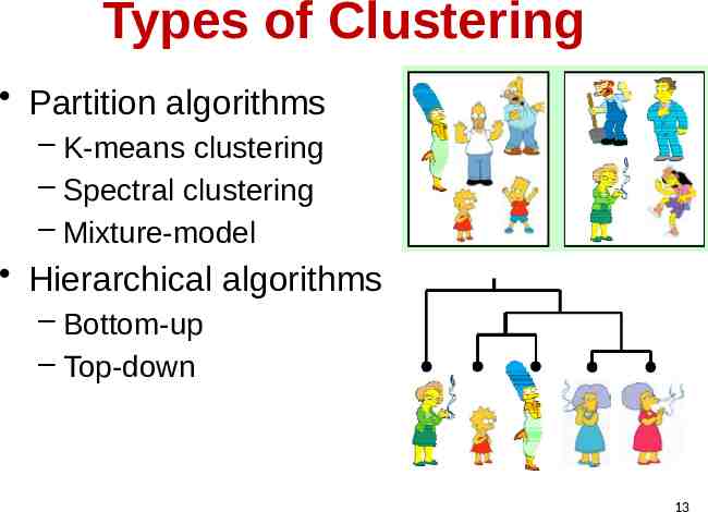
Types of Clustering Partition algorithms – K-means clustering – Spectral clustering – Mixture-model Hierarchical algorithms – Bottom-up – Top-down 13

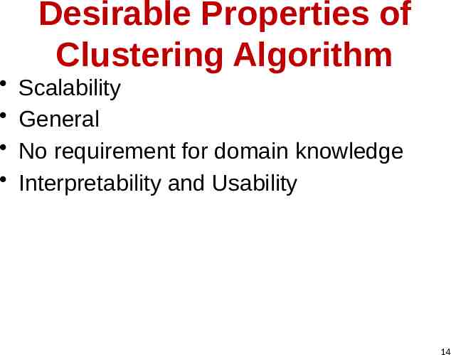
Desirable Properties of Clustering Algorithm Scalability General No requirement for domain knowledge Interpretability and Usability 14

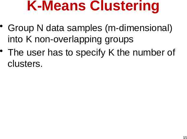
K-Means Clustering Group N data samples (m-dimensional) into K non-overlapping groups The user has to specify K the number of clusters. 15

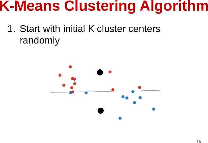
K-Means Clustering Algorithm 1. Start with initial K cluster centers randomly 16

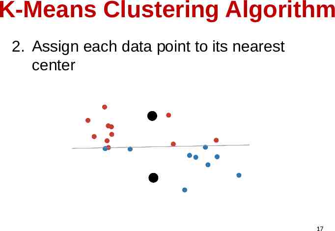
K-Means Clustering Algorithm 2. Assign each data point to its nearest center 17

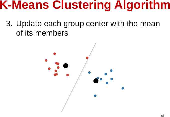
K-Means Clustering Algorithm 3. Update each group center with the mean of its members 18

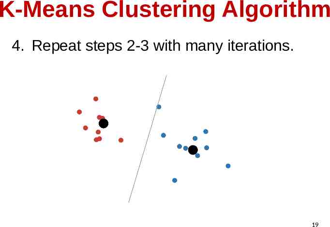
K-Means Clustering Algorithm 4. Repeat steps 2-3 with many iterations. 19

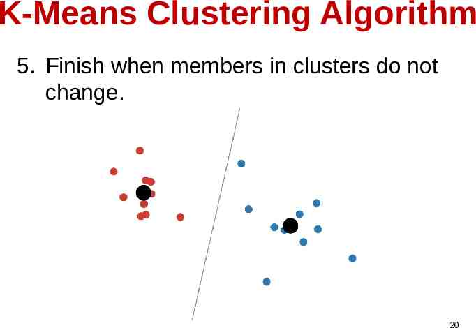
K-Means Clustering Algorithm 5. Finish when members in clusters do not change. 20

K-Means Algorithm 1. Start with initial K cluster centers randomly 2. Assign each data point to its nearest center using distance function 3. Update each group center with the mean of its members 4. Repeat steps 2-3 with many iterations until members in clusters do not change. Demo:https ://www.naftaliharris.com/blog/visualizing-k-m21

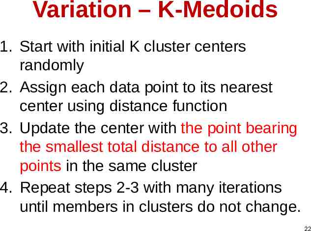
Variation – K-Medoids 1. Start with initial K cluster centers randomly 2. Assign each data point to its nearest center using distance function 3. Update the center with the point bearing the smallest total distance to all other points in the same cluster 4. Repeat steps 2-3 with many iterations until members in clusters do not change. 22

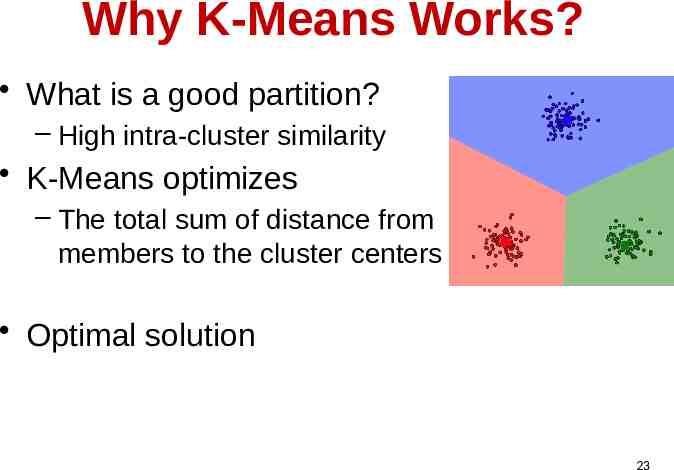
Why K-Means Works? What is a good partition? – High intra-cluster similarity K-Means optimizes – The total sum of distance from members to the cluster centers Optimal solution 23

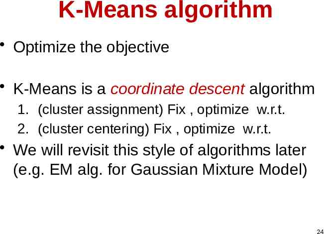
K-Means algorithm Optimize the objective K-Means is a coordinate descent algorithm 1. (cluster assignment) Fix , optimize w.r.t. 2. (cluster centering) Fix , optimize w.r.t. We will revisit this style of algorithms later (e.g. EM alg. for Gaussian Mixture Model) 24

Quiz On Edstem 25

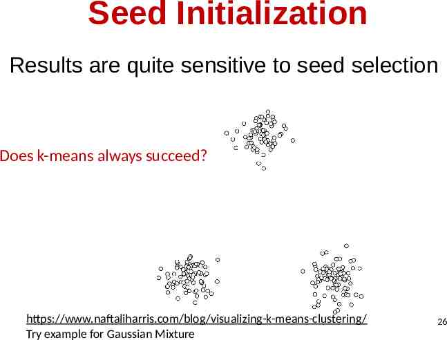
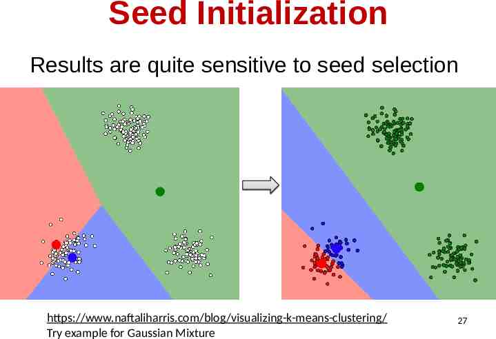
Seed Initialization Results are quite sensitive to seed selection Does k-means always succeed? https://www.naftaliharris.com/blog/visualizing-k-means-clustering/ Try example for Gaussian Mixture 26

Seed Initialization Results are quite sensitive to seed selection https://www.naftaliharris.com/blog/visualizing-k-means-clustering/ Try example for Gaussian Mixture 27

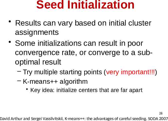
Seed Initialization Results can vary based on initial cluster assignments Some initializations can result in poor convergence rate, or converge to a suboptimal result – Try multiple starting points (very important!!!) – K-means algorithm Key idea: initialize centers that are far apart 28 David Arthur and Sergei Vassilvitskii, K-means : the advantages of careful seeding. SODA 2007

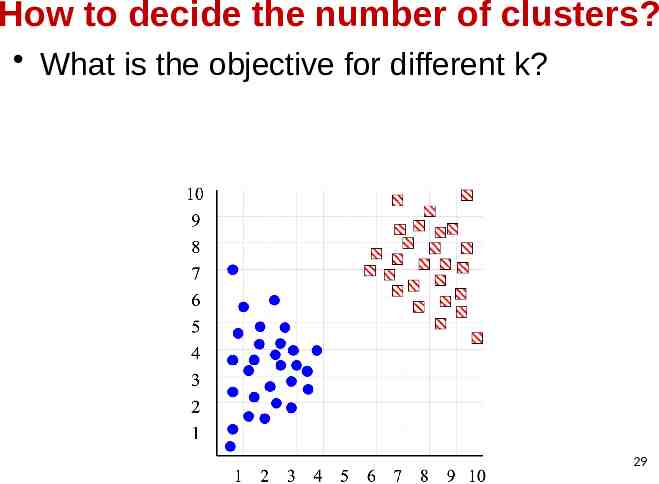
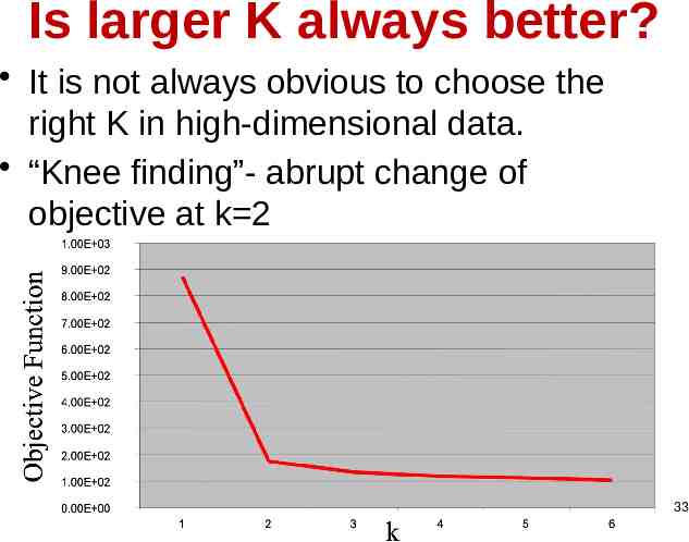
How to decide the number of clusters? What is the objective for different k? 29

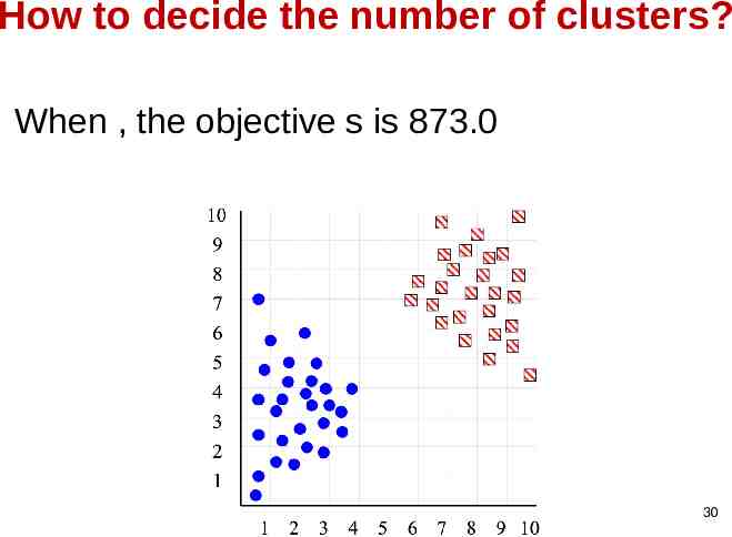
How to decide the number of clusters? When , the objective s is 873.0 30

How to decide the number of clusters? When , the objective s is 173.1 31

How to decide the number of clusters? When , the objective s is 133.6 32

Is larger K always better? It is not always obvious to choose the right K in high-dimensional data. “Knee finding”- abrupt change of objective at k 2 33

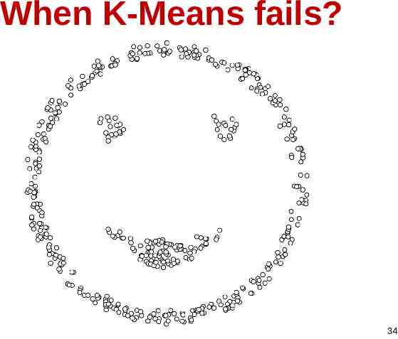
When K-Means fails? 34

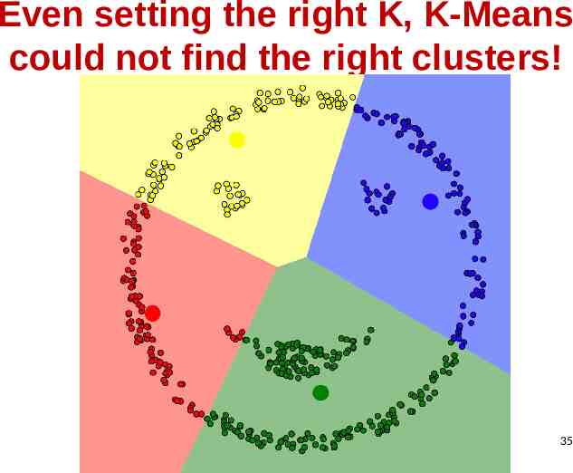
Even setting the right K, K-Means could not find the right clusters! 35

Summary: K-Means Clustering Strength – Simple, easy to implement and debug – Intuitive objective function: optimizing intra-cluster similarity – Efficient: complexity ? Weakness – Applicable only when mean can be calculated What about Categorical data? – – – – Terminates at a local optimum. Initialization is important Sensitive to noisy data and outliers Not able to find clusters with non-convex shape 36

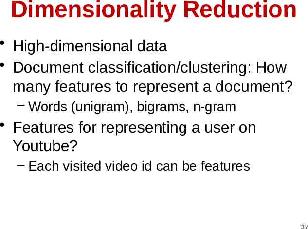
Dimensionality Reduction High-dimensional data Document classification/clustering: How many features to represent a document? – Words (unigram), bigrams, n-gram Features for representing a user on Youtube? – Each visited video id can be features 37

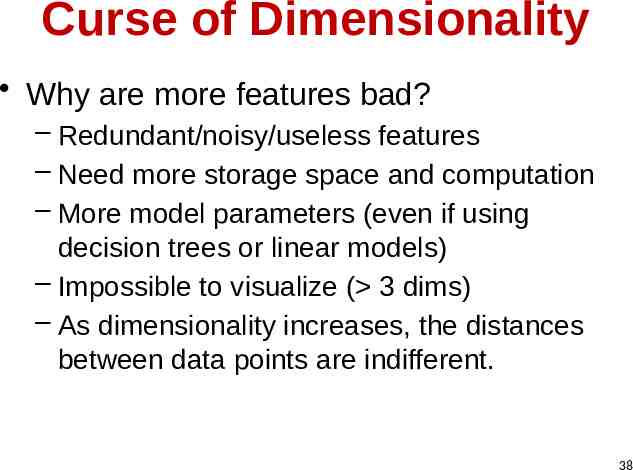
Curse of Dimensionality Why are more features bad? – Redundant/noisy/useless features – Need more storage space and computation – More model parameters (even if using decision trees or linear models) – Impossible to visualize ( 3 dims) – As dimensionality increases, the distances between data points are indifferent. 38

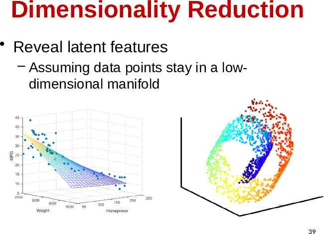
Dimensionality Reduction Reveal latent features – Assuming data points stay in a lowdimensional manifold 39

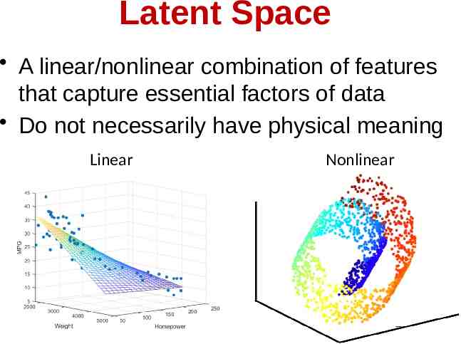
Latent Space A linear/nonlinear combination of features that capture essential factors of data Do not necessarily have physical meaning Linear Nonlinear 40

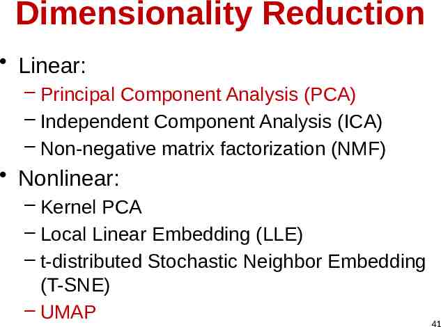
Dimensionality Reduction Linear: – Principal Component Analysis (PCA) – Independent Component Analysis (ICA) – Non-negative matrix factorization (NMF) Nonlinear: – Kernel PCA – Local Linear Embedding (LLE) – t-distributed Stochastic Neighbor Embedding (T-SNE) – UMAP 41

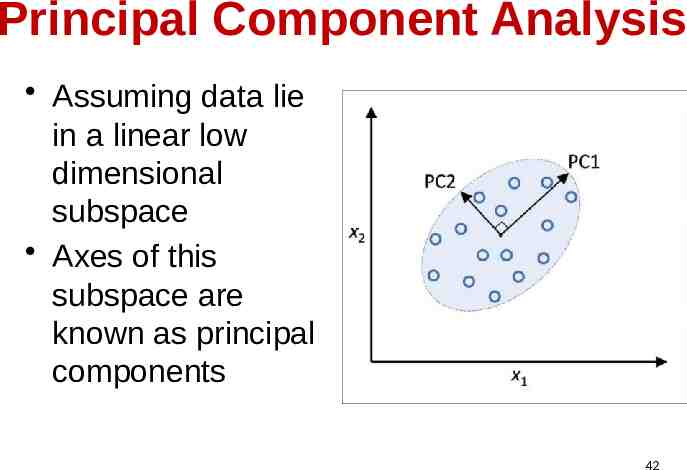
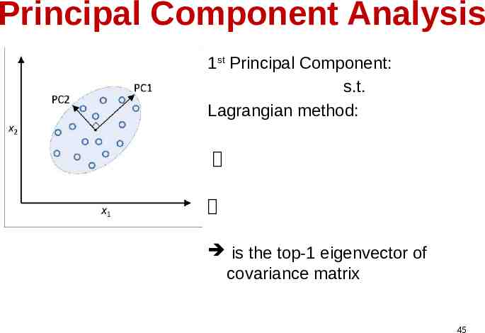
Principal Component Analysis Assuming data lie in a linear low dimensional subspace Axes of this subspace are known as principal components 42

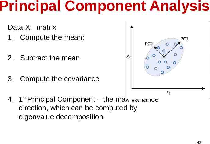
Principal Component Analysis Data X: matrix 1. Compute the mean: 2. Subtract the mean: 3. Compute the covariance 4. 1st Principal Component – the max variance direction, which can be computed by eigenvalue decomposition 43

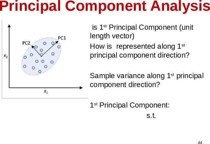
Principal Component Analysis is 1st Principal Component (unit length vector) How is represented along 1st principal component direction? Sample variance along 1st principal component direction? 1st Principal Component: s.t. 44

Principal Component Analysis 1st Principal Component: s.t. Lagrangian method: is the top-1 eigenvector of covariance matrix 45

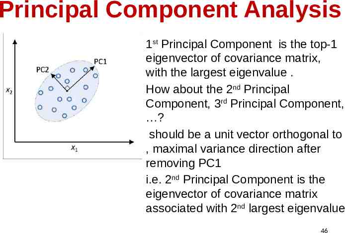
Principal Component Analysis 1st Principal Component is the top-1 eigenvector of covariance matrix, with the largest eigenvalue . How about the 2nd Principal Component, 3rd Principal Component, ? should be a unit vector orthogonal to , maximal variance direction after removing PC1 i.e. 2nd Principal Component is the eigenvector of covariance matrix associated with 2nd largest eigenvalue 46

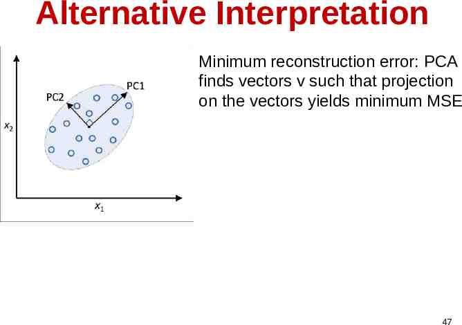
Alternative Interpretation Minimum reconstruction error: PCA finds vectors v such that projection on the vectors yields minimum MSE 47

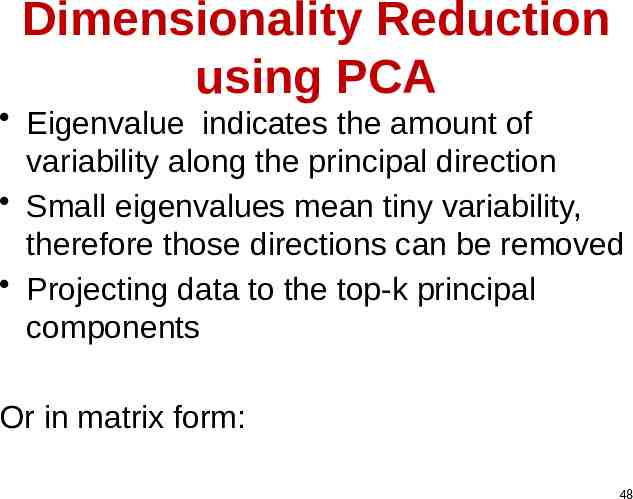
Dimensionality Reduction using PCA Eigenvalue indicates the amount of variability along the principal direction Small eigenvalues mean tiny variability, therefore those directions can be removed Projecting data to the top-k principal components Or in matrix form: 48

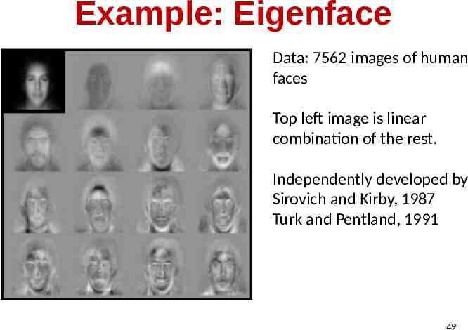
Example: Eigenface Data: 7562 images of human faces Top left image is linear combination of the rest. Independently developed by Sirovich and Kirby, 1987 Turk and Pentland, 1991 49

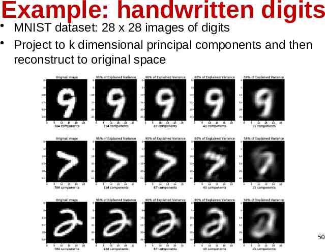
Example: handwritten digits MNIST dataset: 28 x 28 images of digits Project to k dimensional principal components and then reconstruct to original space 50

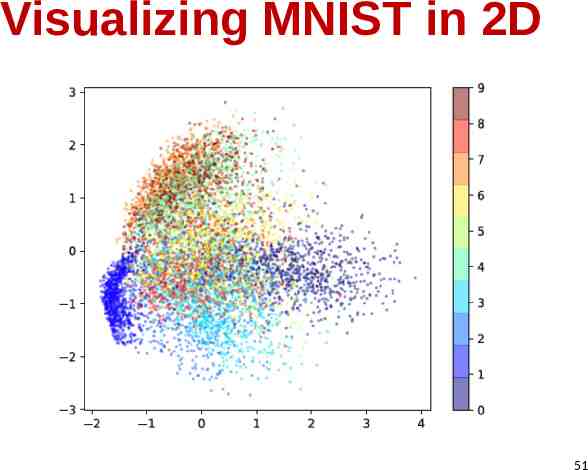
Visualizing MNIST in 2D 51

Interactive Illustration https://setosa.io/ev/principal-component-ana lysis/ 52

Properties of PCA Advantage: – Eigen decomposition, O(n3) – No need to tune parameters Weaknesses – Linear projection – Second-order statistics (covariance) 53

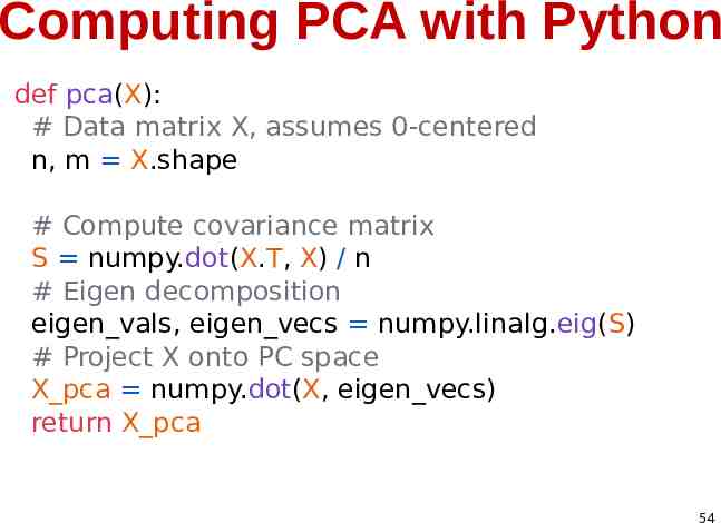
Computing PCA with Python def pca(X): # Data matrix X, assumes 0-centered n, m X.shape # Compute covariance matrix S numpy.dot(X.T, X) / n # Eigen decomposition eigen vals, eigen vecs numpy.linalg.eig(S) # Project X onto PC space X pca numpy.dot(X, eigen vecs) return X pca 54

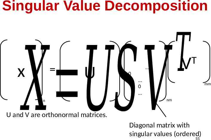
Singular Value Decomposition 𝑋 𝑈𝑆𝑉 0 x U n 0 0 n 𝑇 V T mm nm U and V are orthonormal matrices. Diagonal matrix with singular values (ordered) 55

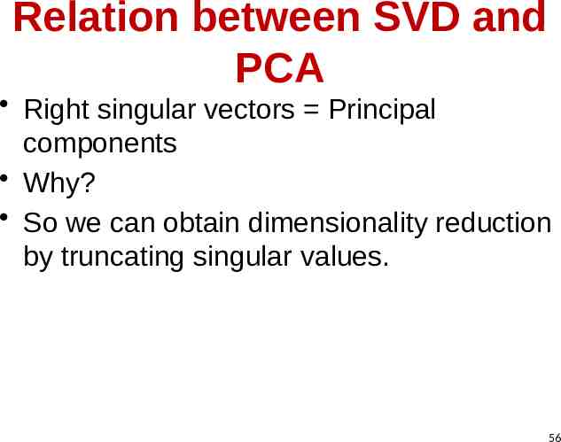
Relation between SVD and PCA Right singular vectors Principal components Why? So we can obtain dimensionality reduction by truncating singular values. 56

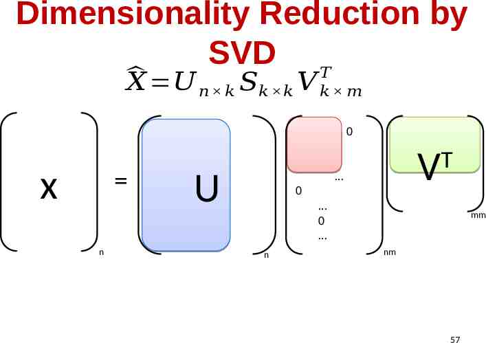
Dimensionality Reduction by SVD 𝑇 𝑋 𝑈 𝑛 𝑘 𝑆𝑘 𝑘 𝑉 𝑘 𝑚 0 x n U V T 0 0 n mm nm 57

SVD and PCA PCA can be computed using SVD Computing SVD with top-k singular values is faster than PCA with eigen decomposition. SVD can be used to compute the pseudoinverse of a rectangular matrix 58

Summary: Dimensionality Reduction Principal Component Analysis 1. 2. 3. 4. Center the data by subtracting the mean Compute covariance matrix Eigen decomposition on covariance matrix Eigenvectors are principal components, eigenvalues are energy Singular Value Decomposition – Can be used to compute PCA, and faster – Reduce the dimension by truncating at top-k singular values. 59